Neural network does quantum mechanics

A particle confined to an impassable box is a paradigmatic and exactly solvable one-dimensional quantum system modeled by an infinite square well potential. Working with Bill Ditto, Elliott Holliday and I recently explored some of its infinitely many generalizations to two dimensions, including particles confined to regions that exhibit integrable, ergodic, or chaotic classical billiard dynamics, using physics-informed neural networks. In particular, we generalized an unsupervised learning algorithm to find the particles’ eigenvalues and eigenfunctions, even in cases where the eigenvalues are degenerate. During training, the neural network adjusts its weights and biases, one of which is the energy eigenvalue, so that its output approximately solves the stationary Schrödinger equation with normalized and mutually orthogonal eigenfunctions.


2D classical billiard orbits and corresponding 2nd quantum eigenfunctions

2D classical billiard orbits (left) and corresponding 2nd quantum eigenfunctions (right)

Posted in Physics | Leave a comment

The Ringed Planets

When I was a kid, Saturn was the ringed planet. But today, we know that all of the outer planets have rings. The James Webb Space Telescope has now imaged each of them in infrared revealing their distinctive structures, including Jupiter‘s very faint ring (located by the arrow and dashed curve). The planet images below are roughly to scale, 11:9:4:4, where Earth is 1.


Jupiter

Saturn

Uranus

Neptune

Posted in Astronomy | Leave a comment

Simplest Chaos

The motion of one of the simplest dynamical systems, a torqued, damped, nonlinear pendulum, can be infinitely complicated.

Consider a simple pendulum of length l and mass m rigidly connected to an axle of radius r wrapped by a rope that hangs down one side with a mass M climbing up and down it, as in the attached animation.

If the climber’s height

x = x_0  + \frac{a}{\omega^2} \sin \omega t,

varies sinusoidally (relative to the axle), then its acceleration

\ddot x = - a \sin \omega t,

also varies sinusoidally, so the total force on the climber

M\ddot x = \sum_\text{down} f = Mg-T

implies upper rope tension

T = Mg + ma \sin \omega t,

where 0 < a < g. If the axle and rope have negligible inertia, then the total torque on the axle

m l^2 \ddot \theta = \sum_\text{CCW}\tau = - mgl \sin\theta + rT - \gamma \dot\theta,

where \gamma is the axle viscosity. The full motion equation

m l^2 \ddot \theta = - mgl \sin\theta + rMg + rma \sin \omega t - \gamma \dot\theta

reduces to

\ddot \theta = - \sin\theta + 0.7155 + 0.4 \sin 0.25 t - 0.75 \dot\theta

for parameters that describe the animation’s chaotic motion.


Mass sinusoidally climbs up and down brown rope torquing blue pendulum into chaotic motion

Green mass sinusoidally climbs up and down brown rope torquing blue pendulum into chaotic motion. Upper rope tension is largest with climber lowest and smallest with climber highest.

Posted in Physics | Leave a comment

Vampire Ein Stein

Just a couple of months after announcing the remarkable discovery of a single shape that forces a non-periodic tiling of the plane, Smith, Myers, Kaplan, and Goodman-Strauss have announced an improved aperiodic monotile or ein stein. (Ein stein is “one stone” in German.)


Aperiodic tilings


The hat and turtle shapes tile the plane only non-periodically, but with their mirror reflections, which would be practically troublesome for one-sided tiles. Smith and colleagues realized that if reflections are forbidden an intermediate equilateral shape tiles the plane only non-periodically. Furthermore, perturbing the shape’s sides can block periodic tiling using it and its reflection, thereby generating specter shapes that tile the plane only non-periodically, whether reflections are allowed or forbidden.

Because specters don’t need their reflections, and vampires are said to not reflect in mirrors, the authors playfully suggest calling them vampire ein steins. You could tile your bathroom with a single specter shape, even though bathroom tile is glazed on only one side!

Below are three different colorings of a tiling by a stegosaurus shape, a particularly simple equilateral specter with only \pm 60^\circ and \pm 90^\circ turns (and a single 0^\circ turn), which I created in Mathematica and Illustrator. The darker tile pairs in the first coloring are called mystics


Aperiodic tiling 2

Posted in Mathematics | Leave a comment

The Temperature of the Vacuum

Quantum field theory predicts that the temperature of empty space should depend on the observer’s motion, increasing proportionally with acceleration. Here I attempt an accessible introduction to this striking effect, related to Hawking radiation and discovered independently by Fulling, Davies, and Unruh, assuming only sophomore-level physics (including hyperbolic functions) with some assistance from Mathematica.

Hyperbolic Motion

Constant acceleration in Newtonian mechanics is parabolic, while constant acceleration in Einsteinian mechanics is hyperbolic and asymptotic to light speed c = 1 in natural units. For 1+1-dimensional Minkowski spacetime, the difference in squared space and time displacements is the square of proper time displacement,

d\tau^2 = dt^2 - dx^2.

For constant proper acceleration, this has the solution

dt = d\tau \cosh a\tau,vdx = d\tau \sinh a\tau,
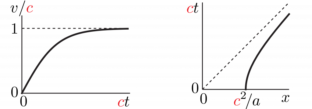
with velocity

v = \frac{dx}{dt} = \tanh a\tau \le 1,

where for small times v \sim a \tau \sim a t. If t = 0 and a x = 1 at \tau = 0, then integration gives

a t = \sinh a \tau,\\a x = \cosh a\tau.

Hyperbolic identities then imply

a^2 x^2 - a^2 t^2 = 1

and

a x + a t = e^{a\tau}.


Position and speed for hyperbolic motion

Quantum Vacuum

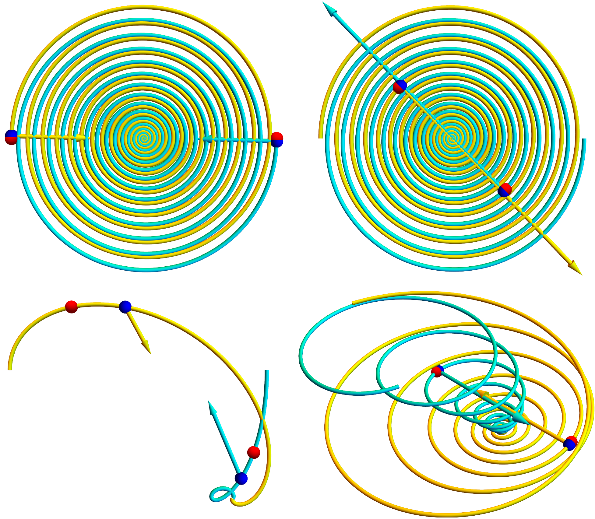
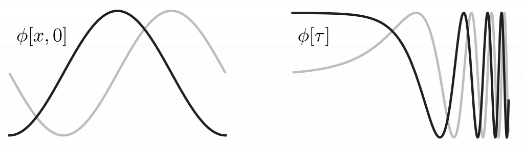
Due to Heisenberg indeterminacy, electromagnetic fluctuations fill the vacuum. Consider a single such sinusoidal wave of angular frequency \omega_0 = k_0 in natural units. If you move at constant velocity, you observe the wave doppler-shifted to a different frequency. But if you move at constant acceleration, you observe the wave doppler-shifted to a range of frequencies corresponding to your range of velocities. For an accelerated observer at time \tau,

\phi[x,t] = \exp\left[i(k_0 x + \omega_0 t)\right] = \exp\left[i\omega_0(x + t)\right] \\= \exp\left[{i \frac{\omega_0}{a} e^{a \tau}} \right] = \phi[\tau].


Sinusoidal waveforms


Expand this waveform as a sum of harmonics

\phi[\tau] = \int_{-\infty}^{\infty}\,\frac{d\omega}{2\pi} \Phi[\omega] \exp[-i \omega \tau]

where the Fourier components

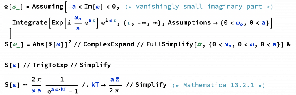
\Phi[\omega] = \int_{-\infty}^{\infty}d\tau\, \phi[\tau] \exp[+i \omega \tau].

To regularize this divergent integral, subtract a tiny imaginary part i \epsilon from the angular frequency \omega to incorporate a decaying exponential factor e^{-\epsilon \tau} in the integrand, and zero it after integrating. Find

\Phi[\omega] = \lim_{\epsilon\rightarrow 0} \int_{-\infty}^{\infty}d\tau\, \exp\left[ i \frac{\omega_0}{a} e^{a\tau} \right] \exp[+i (\omega - i \epsilon) \tau]\\~ \\= \lim_{\epsilon\rightarrow 0}\, \exp\left[ i\frac{\pi}{2} \left(\frac{\epsilon + i\omega}{a}\right) \right]\left(\frac{a}{\omega_0}\right)^{(\epsilon + i \omega)/a}\frac{1}{a} \Gamma\left[\frac{\epsilon + i \omega}{a} \right] \\= \exp\left[-\frac{\pi}{2} \frac{\omega}{a}\right]\left(\frac{a}{\omega_0}\right)^{i \omega / a}\frac{1}{a} \Gamma\left[i \frac{\omega}{a} \right],

where \Gamma[n+1] = n! analytically continues the factorial function to the complex plane. The spectrum is the absolute square of the Fourier transform,

S[\omega] = \left|\Phi[\omega]\right|^2 = \frac{\pi}{a\omega} \left(\coth\left[ \pi \frac{\omega}{a} \right]-1 \right) \\= \frac{2\pi}{\omega a} \frac{1}{e^{2\pi \omega/a} - 1} \propto \frac{1}{e^{\hbar \omega/k T}-1},

where the Planck factor suggests Bose-Einstein statistics and a thermal photon bath of temperature kT = a \hbar / 2\pi. In SI units,

T = \frac{a \hbar}{2\pi k c} \sim 40~\text{zK}~\left(\frac{a}{g_E} \right),

where g_E is Earth’s surface gravity, and a zeptokelvin is very cool.


Mathematica check

Hawking-Unruh Temperature

Just prior to the 1970s work of Fulling, Davies, and Unruh, Stephen Hawking famously predicted that despite their reputations black holes should radiate with an effective temperature

T = \frac{\kappa \hbar}{2\pi k c},

where \kappa is the black hole’s surface gravity (observed at infinity). The Unruh and Hawking results may be linked by the equivalence principle, which equates acceleration and gravity, and by event horizons. In General Relativity, the black hole horizon is a boundary that causally disconnects the interior from the exterior. Similarly, when you accelerate, a Rindler horizon appears a distance c^2/a \sim 1~\text{ly} \left(g_E / a \right) behind you, causally disconnecting you from a region of spacetime whose photons you can outrun (so long as your acceleration continues).

Posted in Physics | Leave a comment

A Century of Compton Scattering

One hundred years ago today the Physical Review published research on light scattering electrons that would earn its author, Wooster graduate Arthur Compton, a Physics Nobel Prize.

By relativistically conserving spacetime momentum, as in the diagram below, and treating light as particles now called photons, Compton discovered that deflecting an electron through an angle \theta stretches the light’s wavelength by

\frac{ \Delta \lambda}{\lambda_c} = 1 - \cos\theta,

where \lambda_c = h / mc \sim 1/40 \textup{~\AA} is the Compton wavelength of the electron. Compton’s experiment helped convince the physics community of wave-particle duality. Today, sophomores Compton scatter in our Modern Physics lab.


2+1 dimensional Compton scattering diagram

Compton scattering of a photon (blue to red) from an electron (green) in space (bottom) and spacetime (top). The photon lives on the light cones while the electron lives in the light cones.

Posted in Physics, Wooster | Leave a comment

We Are Going

After half a century confined to low-Earth orbit, and as soon as late next year, humans will once again leave Earth and voyage to Moon. The reality of this exciting adventure crystallized earlier this month when NASA announced the diverse and inspiring Artemis II crew: Clockwise from left in the photo below are Christina Koch, Victor Glover, Jeremy Hansen, and Reid Wiseman.

Christina holds the record for longest space flight by a woman, during which she participated in the first all-woman spacewalk. She is now scheduled to become the first woman to fly around Moon. Along with two electrical engineer degrees, Christina obtained a bachelor’s degree in physics from NC State, and I often think of her as I walk to my present office in NC State’s physics building (although I understand that physics moved into the renovated Riddick shortly after she graduated).


Group portrait of Christina Koch, Victor Glover, Jeremy Hansen, Reid Wiseman, the crew of Artemis II

Christina Koch, Victor Glover, Jeremy Hansen, Reid Wiseman, the crew of Artemis II. (Photo by Josh Valcarcel for NASA.)

Posted in Adventure, Physics, Space Exploration | Leave a comment

Behold, an Ein Stein!

This academic year has been thrilling: first nuclear fusion breakeven, now an ein stein!

Last week, a preprint at arxiv.org by David Smith et al. announced an “ein stein”, or one stone, a shape that forces a non periodic tiling of the plane, ending a half-century quest by many researchers, including me. A retiree and tiling enthusiast, Smith discovered the shape, which he calls “the hat”, and his professional colleagues provided mathematical and computational rigor.

In the 1960s, Robert Berger found a set of 20 426 tile-types that tile a plane but only non periodically — a wonderful mix of the expected and the surprising, a kind of visual music. By the 1970s, Roger Penrose has reduced that to just 2 tile-types, but a further reduction to just 1 tile-type proved elusive. Of Smith’s hat, the 91-year-old Roger Penrose reportedly observed, “It’s a really good shape, strikingly simple”, and I agree.

In the grayscale figure below, an underlying hexagonal grid emphasizes the hat’s construction. Given the prior theoretical and computational work that failed to find it, the hat is a surprisingly simple polykite formed from 8 kites or 4 double kites. In the color figure below, I color the hats according to their orientations (brightnesses) and reflections (hues), something I’ve dreamed of doing for many years, even in the absence of an ein stein.

You could order many flat paving stones shaped like the hat and translate, rotate, and flip them to non periodically tile your patio. I just might.

Figure 1.1 from David Smith et al. 'An aperiodic monotile' emphasizing the underlying hexagonal foundation of 'the hat', which is a tridecagon made from 8 kites or 4 double kites.

Figure 1.1 from David Smith et al. “An aperiodic monotile” emphasizing the underlying hexagonal foundation of “the hat”, which is a tridecagon made from 8 kites or 4 double kites.

The hat forces a non periodic tiling of the plane, where brightnesses indicate 1 of 6 orientations and hues indicate 1 of 2 reflections.

The hat forces a non periodic tiling of the plane, where brightnesses indicate 1 of 6 orientations and hues indicate 1 of 2 reflections. (Alternately, the orientations and reflections can all be considered rotations about axes perpendicular or parallel to the plane.)

Posted in Mathematics | Leave a comment

Generalizing Coulomb’s Law

The forces between two electric charges in arbitrary motion are complicated by velocity, acceleration, and time-delay effects. The forces need not even lie along the line joining the two charges!

Suppose a source charge q^\prime is at position \vec r^{\,\prime} with velocity \vec v^{\,\prime} and acceleration \vec{a}^{\,\prime}, and a test charge q is at position \vec r with velocity \vec v and acceleration \vec{a}. Let their separation \vec{\mathcal{R}}= \vec r - \vec r^{\,\prime}. Since electromagnetic “news” travels at light speed \color{blue}c\color{black} = 1 (in natural units), define the earlier retarded time s < t  implicitly by t - s = \mathcal{R}[s] / \color{blue}c\color{black} = \mathcal{R}_{\color{red}s}.

Liénard-Wiechert electric and magnetic potentials at test charge q due to source charge q^\prime are

\varphi_{\color{red}t} =\frac{q^\prime_e}{4\pi \mathcal{R}_{\color{red}s} }=\frac{q^\prime}{4\pi \mathcal{R}_{\color{red}s} } \left( \frac{1}{1 - \hat{\mathcal{R} }_{\color{red}s} \cdot \vec v^{\,\prime}_{\color{red}s}} \right), \hspace{1cm} \vec A_{\color{red}t}= \varphi^\prime_{\color{red}s} \vec v^{\,\prime}_{\color{red}s},

where the source charge q^\prime is “smeared” to an effective charge q^\prime_e by its motion, and the subscripts indicate evaluation times. If the source charge velocity \vec v^{\,\prime}_{\color{red}s} = 0, then the potentials simplify to the electrostatics limit. Differentiate the potentials to find Maxwell’s electric and magnetic fields

\vec{\mathcal{E}} = - \vec \nabla \varphi - \partial_t \vec A \hspace{1cm} \vec{\mathcal{B}} = \vec \nabla \times \vec A,

and the Lorentz force law

\vec F = q \left( \vec{\mathcal E} + \vec v \times \vec{\mathcal B}\right)

generalizes Coulomb’s law to

\vec F_{\color{red}t} = q \frac{ q^\prime } { 4 \pi \mathcal{R}^2_{\color{red}s}} \left( \frac{ 1 } {1 - \hat{\mathcal{R}}_{\color{red}s} \cdot \vec{v}^{\,\prime}_{\color{red}s} }\right)^3 \bigg( \frac{}{} (1-v^{\prime 2}_{\color{red}s})(\hat{\mathcal{R}}_{\color{red}s}-\vec{v}^{\,\prime}_{\color{red}s}) + \vec{\mathcal{R}}_{\color{red}s} \times \left((\hat{\mathcal{R}}_{\color{red}s}-\vec{v}^{\,\prime}_{\color{red}s}) \times \vec{a}^{\,\prime}_{\color{red}s} \right) \hspace{3.4cm} + \,\vec v_{\color{red}t} \times \left( \hat{\mathcal{R}}_{\color{red}s} \times \left( (1-v^{\prime 2}_{\color{red}s})(\hat{\mathcal{R}}_{\color{red}s}-\vec{v}^{\,\prime}_{\color{red}s}) + \vec{\mathcal{R}}_{\color{red}s} \times \left((\hat{\mathcal{R}}_{\color{red}s}-\vec{v}^{\,\prime}_{\color{red}s}) \times \vec{a}^{\,\prime}_{\color{red}s} \right) \right) \right) \, \bigg).

If the test charge velocity \vec v = \vec 0, then the magnetic terms vanish; if the source charge acceleration \vec{a}^{\,\prime} = \vec 0, then the radiation terms vanish; if, in addition, the source charge velocity \vec v\,^\prime = \vec 0, then the generalized Coulomb’s law reduces to the familiar electrostatic limit. Finally, Newton’s second law with Einstein’s momentum

\vec F = \frac{d\vec p}{dt} = \frac{d}{dt} \frac{ m \vec v }{\sqrt{1 - v^2}} = \frac{ m \vec a}{\sqrt{1 - v^2}} + \frac{ m \vec v}{(1 - v^2)^{3/2}} \vec v \cdot \vec a

generates the motion equations using 3-vectors and lab time (instead of 4-vectors and proper time), succinctly summarizing all of electromagnetism.

Using Mathematica, I eliminated present time t from the motion equations with the substitution t = s + \mathcal{R}_{\color{red}s} and numerically integrated them with respect to the retarded time s for various initial conditions, as in the figure below. Positive and negative charge pairs tugged by non-zero net forces spiral into one another as they radiate away energy and momentum, graphically demonstrating the instability of classical atoms.

Mathematica simulations of interacting charged particle including magnetic, radiation, and time-delay effects. Blue dots mark present positions, and red dots mark retarded positions. Arrows represent force pairs, which are typically not "equal but opposite".

Mathematica simulations of interacting charged particle including magnetic, radiation, and time-delay effects. Blue dots mark present positions, and red dots mark retarded positions. Arrows represent force pairs, which are typically not “equal but opposite”.

Posted in Physics | Leave a comment

Wooster Physics Alumni at Kent Displays

Three Wooster physics alumni who all work at Kent Displays, Inc. returned to campus last Thursday to share some info about the physics of liquid crystals as well as some of their personal journeys to Wooster and beyond.

See more information over at the NEWS page on the Wooster Physics website!

Posted in Fun, Physics, Students, Wooster | Leave a comment