
The forces between two electric charges in arbitrary motion are complicated by velocity, acceleration, and time-delay effects. The forces need not even lie along the line joining the two charges!
Suppose a source charge q^\prime is at position \vec r^{\,\prime} with velocity \vec v^{\,\prime} and acceleration \vec{a}^{\,\prime}, and a test charge q is at position \vec r with velocity \vec v and acceleration \vec{a}. Let their separation \vec{\mathcal{R}}= \vec r – \vec r^{\,\prime}. Since electromagnetic “news” travels at light speed \color{blue}c\color{black} = 1 (in natural units), define the earlier retarded time s < t implicitly by t – s = \mathcal{R}[s] / \color{blue}c\color{black} = \mathcal{R}_{\color{red}s}.
Liénard-Wiechert electric and magnetic potentials at test charge q due to source charge q^\prime are
\varphi_{\color{red}t} =\frac{q^\prime_e}{4\pi \mathcal{R}_{\color{red}s} }=\frac{q^\prime}{4\pi \mathcal{R}_{\color{red}s} } \left( \frac{1}{1 – \hat{\mathcal{R} }_{\color{red}s} \cdot \vec v^{\,\prime}_{\color{red}s}} \right), \hspace{1cm} \vec A_{\color{red}t}= \varphi^\prime_{\color{red}s} \vec v^{\,\prime}_{\color{red}s},where the source charge q^\prime is “smeared” to an effective charge q^\prime_e by its motion, and the subscripts indicate evaluation times. If the source charge velocity \vec v^{\,\prime}_{\color{red}s} = 0, then the potentials simplify to the electrostatics limit. Differentiate the potentials to find Maxwell’s electric and magnetic fields
\vec{\mathcal{E}} = – \vec \nabla \varphi – \partial_t \vec A \hspace{1cm} \vec{\mathcal{B}} = \vec \nabla \times \vec A,and the Lorentz force law
\vec F = q \left( \vec{\mathcal E} + \vec v \times \vec{\mathcal B}\right)generalizes Coulomb’s law to
\vec F_{\color{red}t} = q \frac{ q^\prime } { 4 \pi \mathcal{R}^2_{\color{red}s}} \left( \frac{ 1 } {1 – \hat{\mathcal{R}}_{\color{red}s} \cdot \vec{v}^{\,\prime}_{\color{red}s} }\right)^3 \bigg( \frac{}{} (1-v^{\prime 2}_{\color{red}s})(\hat{\mathcal{R}}_{\color{red}s}-\vec{v}^{\,\prime}_{\color{red}s}) + \vec{\mathcal{R}}_{\color{red}s} \times \left((\hat{\mathcal{R}}_{\color{red}s}-\vec{v}^{\,\prime}_{\color{red}s}) \times \vec{a}^{\,\prime}_{\color{red}s} \right) \hspace{3.4cm} + \,\vec v_{\color{red}t} \times \left( \hat{\mathcal{R}}_{\color{red}s} \times \left( (1-v^{\prime 2}_{\color{red}s})(\hat{\mathcal{R}}_{\color{red}s}-\vec{v}^{\,\prime}_{\color{red}s}) + \vec{\mathcal{R}}_{\color{red}s} \times \left((\hat{\mathcal{R}}_{\color{red}s}-\vec{v}^{\,\prime}_{\color{red}s}) \times \vec{a}^{\,\prime}_{\color{red}s} \right) \right) \right) \, \bigg).If the test charge velocity \vec v = \vec 0, then the magnetic terms vanish; if the source charge acceleration \vec{a}^{\,\prime} = \vec 0, then the radiation terms vanish; if, in addition, the source charge velocity \vec v\,^\prime = \vec 0, then the generalized Coulomb’s law reduces to the familiar electrostatic limit. Finally, Newton’s second law with Einstein’s momentum
\vec F = \frac{d\vec p}{dt} = \frac{d}{dt} \frac{ m \vec v }{\sqrt{1 – v^2}} = \frac{ m \vec a}{\sqrt{1 – v^2}} + \frac{ m \vec v}{(1 – v^2)^{3/2}} \vec v \cdot \vec agenerates the motion equations using 3-vectors and lab time (instead of 4-vectors and proper time), succinctly summarizing all of electromagnetism.
Using Mathematica, I eliminated present time t from the motion equations with the substitution t = s + \mathcal{R}_{\color{red}s} and numerically integrated them with respect to the retarded time s for various initial conditions, as in the figure below. Positive and negative charge pairs tugged by non-zero net forces spiral into one another as they radiate away energy and momentum, graphically demonstrating the instability of classical atoms.
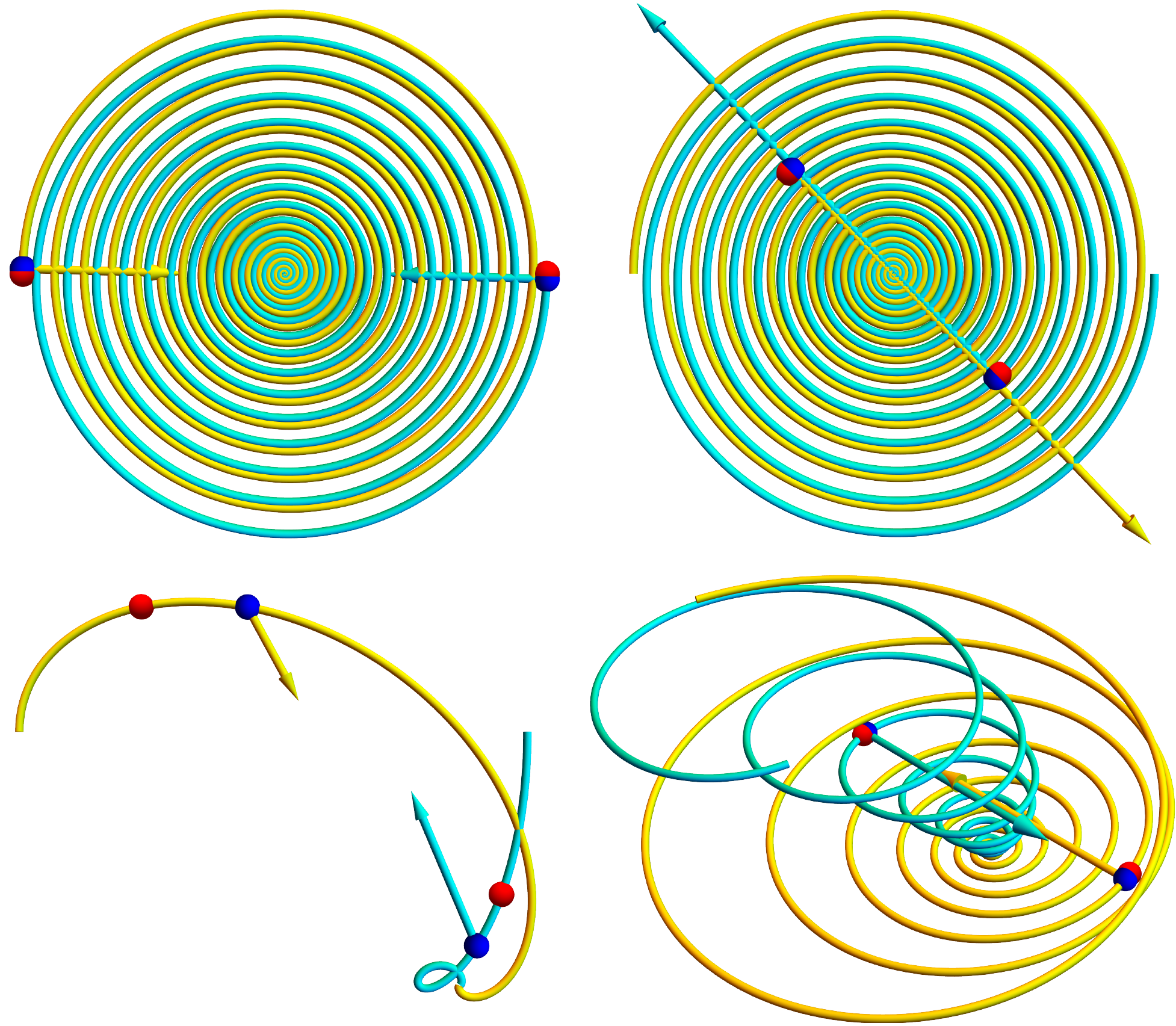
Mathematica simulations of interacting charged particle including magnetic, radiation, and time-delay effects. Blue dots mark present positions, and red dots mark retarded positions. Arrows represent force pairs, which are typically not “equal but opposite”.
Thanks, Mark! I enjoy reading your posts as well.