Artificial neural networks are increasingly important in society, technology, and science, and they are increasingly large and energy hungry. Indeed, the escalating energy footprint of large-scale computing is a growing economic and societal burden. Must we always use brute force, or can we get by with less?
I just co-authored an article in Proceedings of the Royal Society A describing feed-forward neural networks that are small and dynamic, whose nodes can be added (or subtracted) during training. A single neuronal weight in the network controls the network’s size, while the weight itself is optimized by the same gradient-descent algorithm that optimizes the network’s other weights and biases, but with a size-dependent objective or loss function. We trained and evaluated such Nimble Neural Networks on nonlinear regression and classification tasks where they outperform the corresponding static networks, partly because the growing networks have fewer local minima to frustrate the gradient descent.
After explaining conventional neural networks, I provide here an example of one of our growing neural networks.
Conventional Neural Networks
Imagine feed-forward neural networks as interconnected nodes organized in layers, with an input layer, one or more hidden layers, and an output layer. The neurons’ nonlinear activation functions \sigma act on linear combinations of their inputs with the vectorized nested structure
\hat y(x) \overset{\text{vec}}{=} \cdots w^3\sigma(w^2\sigma(w^1 x+b^1 )+b^2)+b^3 \cdots,
where w^l and b^l are the weight matrices and bias vectors of layer l. The weights and biases are free parameters that are tuned during the optimization process.

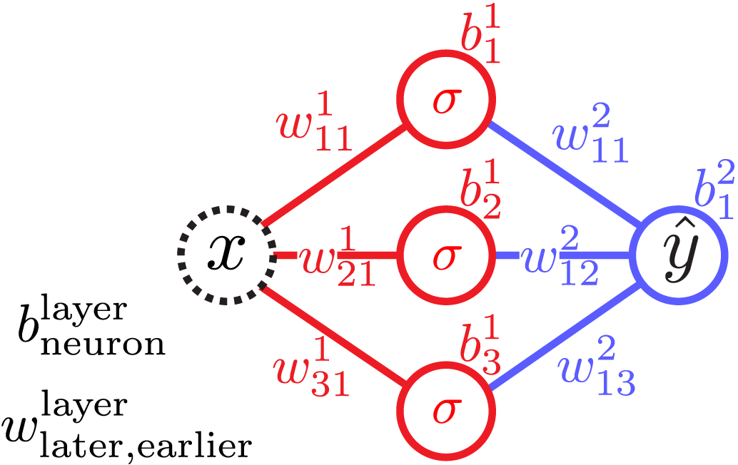
For example, a neural network of 1 input, 1 output, and a single layer of 3 hidden neurons, outputs
\begin{aligned}\hat y(x) = &\color{blue}+w_{11}^2\,\color{red} \sigma\left(w_{11}^1 x + b_1^1 \right) \\ &\color{blue}+w_{12}^2\,\color{red} \sigma \left(w_{21}^1 x + b_2^1 \right) \\ &\color{blue} +w_{13}^2\,\color{red} \sigma \left(w_{31}^1 x + b_3^1 \right) \color{blue}+b_1^2,\end{aligned}
where the weights and biases w^l_{nm} and b^l_n are real numbers. If \sigma(x) = \tanh(x), the special case
\hat y(x) = \sigma(x-6)-\sigma(x-8)
generates the blip

of height 2\tanh(1)\approx 1.5 centered at x = 7 , and combining multiple such blips at different locations with different heights can approximate any reasonable function arbitrarily well, hence the expressive power of neural networks.
An objective or error function, often called a cost or loss function (perhaps from financial applications), \mathcal{L}(x_n,y_n,\hat y(x_n)), quantifies the performance of the network, where \{x_n,y_n\} are the training data. Training attempts to minimize the loss function by repeatedly adjusting the network’s weights and biases. Gradient descent of a neural network weight w can be modeled by a tiny particle of mass m at position x sliding with viscosity \gamma down a potential energy surface V(x), where Newton’s laws imply
m \ddot x = F_x = -\frac{dV}{dx}-\gamma \dot x.
For sufficiently large viscosity (over-damping), the inertial term is negligible, and an Euler update implies
x \leftarrow x + dx = x + \dot x\, dt \sim x- \frac{1}{\gamma} \frac{dV}{dx} dt.
Similarly, with position x = w, height V = \mathcal{L}, and learning rate \eta = dt/\gamma, a neural network weight evolves like
w \leftarrow w-\eta \frac{\partial \mathcal{L}}{\partial w},
and similarly for a bias. While such gradient descent is not guaranteed to find a loss global minimum, it often finds good local minima.
Growing Neural Networks
A size-dependent loss function can drive the network size via gradient descent if the size is identified with an auxiliary weight. An identity activation function with a zero bias converts prepended 1s to the leading weight w^0_{11}, where N = \lfloor w^0_{11} \rfloor is identified with the network size, which gradient descent naturally adjusts along with the other weights and biases.

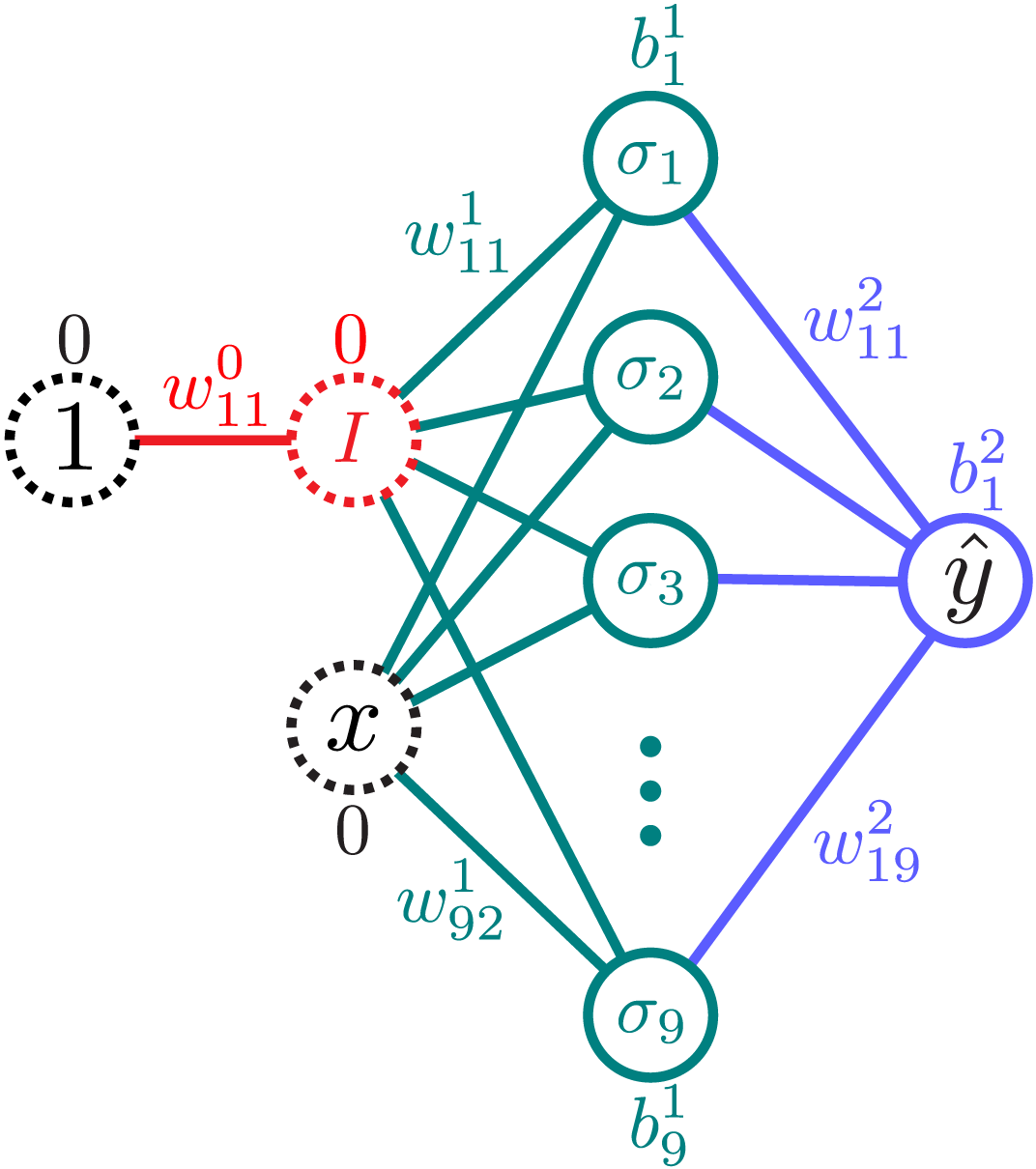
To illustrate the auxiliary-weight algorithm, implement a network with a single hidden layer of up to 9 neurons, with input \mathcal{I}=\{1,x\} and output \mathcal{O} = \hat y, by
\begin{aligned}\hat y(x) = &\color{blue}+w_{11}^2 \color{teal}\sigma_1\big( w_{11}^1 \color{red} I(w_{11}^0 \color{black}1\color{red}+0)\color{teal}+ w_{12}^1 \color{black}x\color{teal}+ b_1^1\big) \\ &\color{blue}+w_{12}^2 \color{teal}\sigma_2\big( w_{21}^1 \color{red} I(w_{11}^0 \color{black}1\color{red}+0)\color{teal}+ w_{22}^1 \color{black}x\color{teal}+ b_2^1\big) \\ &\color{blue}+\cdots \\ &\color{blue}+w_{19}^2 \color{teal}\sigma_9\big( w_{91}^1 \color{red} I(w_{11}^0 \color{black}1\color{red}+0)\color{teal}+ w_{92}^1 \color{black}x\color{teal}+ b_9^1\big)\color{blue}+b_1^2,\end{aligned}
where the identity function I(x) = x, and the possible activation functions
\sigma_r(x) = \theta_r \sigma(x) = \theta_r \tanh(x),
where the C^1 step (down) function
\theta_r = \begin{cases} 1, &\phantom{-1\le} r<-1, \\ \sin^2\left(r \pi / 2\right), & -1\leq r\leq 0, \\ 0, &\phantom{-} 0<r \end{cases}
effectively adds and deletes neurons from the network.
Start with N=0 hidden neurons, so \hat y(x) = b^2_1, and choose a loss function
\mathcal{L} = \mathcal{L}_0+\delta \mathcal{L},
where the base loss varies as the mean-square error
\mathcal{L}_0 = \frac{1}{\mathcal{N}}\sum_{n=1}^{\mathcal{N}} \big(y_n-\hat y(x_n)\big)^2 = \bigg\langle (y-\hat y)^2 \bigg\rangle,
for \mathcal{N} training pairs, which vanishes for perfect agreement y = \hat y, and the size loss
\delta \mathcal{L} = \lambda (N-N_\infty)^2,
which encourages the network to grow to a final size of N = N_\infty hidden neurons. Update the weights and biases, including N = \lfloor w^0_{11} \rfloor, via gradient descent.


Thanks, Mark! I enjoy reading your posts as well.