Saturday, March 8, 2008. A heavy snow, one of the heaviest I remember, shuts down the city of Wooster. Streets are undriveable, so I walk to Taylor Hall, getting snow in my boots.
Taylor is deserted, as the College has begun Spring Break, but like yesterday, Kelly and I work all afternoon and evening in the Physics Shop, me with wet socks. We’re leaving tomorrow, weather permitting, for the New Orleans American Physical Society meeting, where Kelly will present her senior thesis research, but with just hours until our departure, and just days until her I.S. is due, the apparatus is still not working.
Todd brings us sandwiches, which we eat for dinner in the empty Reading Room. Then, just after dinner, back in the shop, the apparatus works for the first time, just as in our computer simulations. But simulation is one thing, reality is another! With no time to celebrate, we video record the dynamics, and move upstairs to the intro physics lab. On one computer, Kelly steps through the video frame-by-frame recording the motion, while at another, I work on the APS poster, which we output with the Taylor large-format printer shortly before midnight.
Next morning is sunny and white, a winter wonderland. The roads are plowed but still snowy. We cautiously drive to the airport and fly to New Orleans via Houston. Kelly’s poster presentation goes well, but I have a fever, sore throat, and stuffy nose. I blame the wet socks.

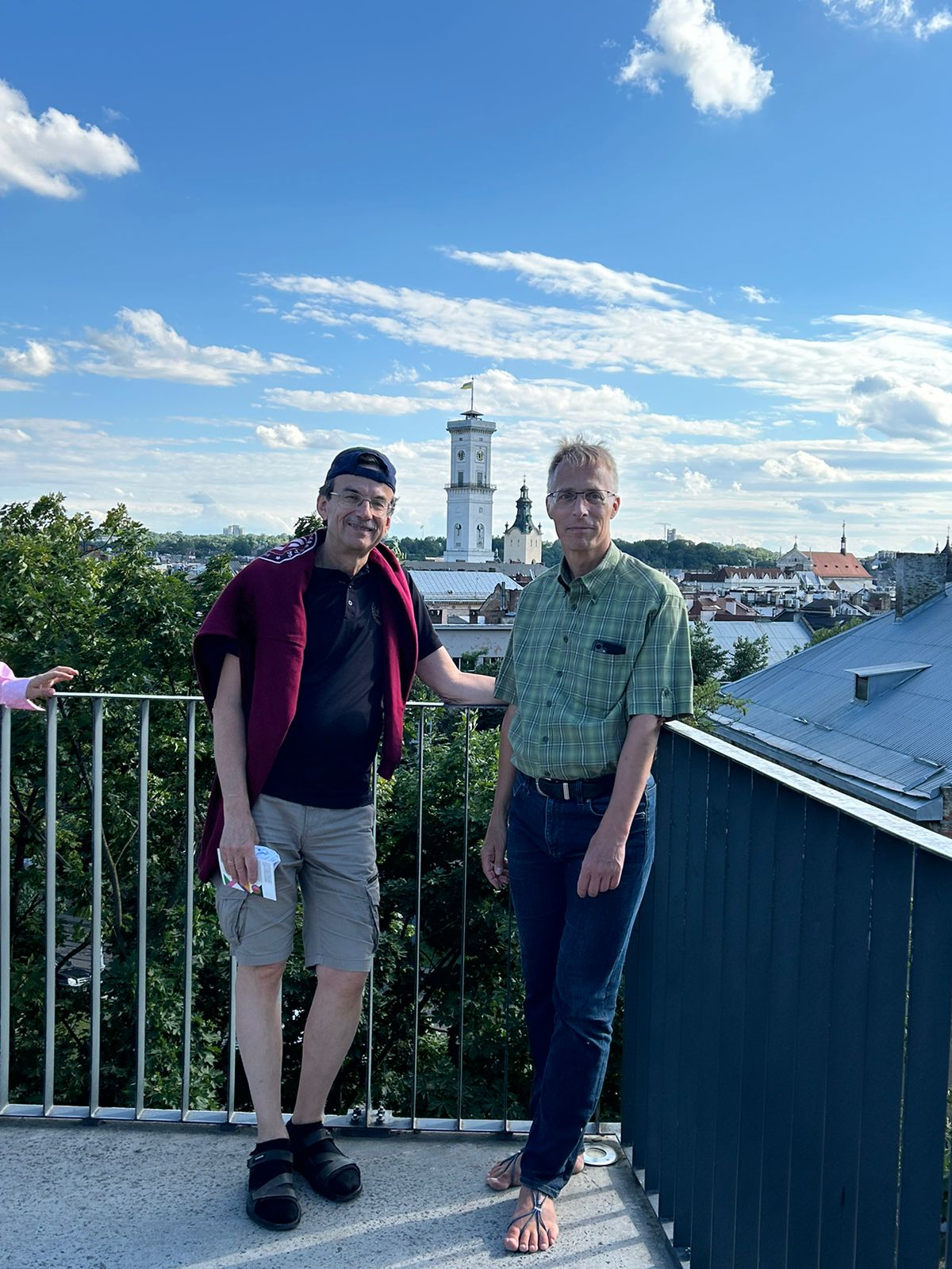
Wooster Physics at the March 2008 APS meeting in New Orleans. Kelly is on the right, and I am next to her. Todd is on the left.
Kelly’s work spawned three publications in refereed journals, two in the Physical Review and one in Chaos, involving many other undergraduates, as we gradually refined the apparatus over the next decade. The final version is on a shelf in my living room beside me as I write this 16 years later.
We designed and constructed a mechanical array of bistable pendulums coupled one-way in a topological ring, so each element affected the next one, but not vice versa, simultaneously violating Newton’s third law of action and reaction, momentum conservation, and energy conservation. Nevertheless, we achieved this by powering the device with a constantly flowing fluid, first water and later air. Each element directed the fluid flow on the next element to rotate it from one stable state to the other.
In this way, solitary waves or solitons of see-sawing elements propagated in one direction along the array, each soliton undoing what the previous one had done. Periodic boundaries enabled solitons to annihilate pairwise in arrays with an even number of elements, but solitons propagated indefinitely in arrays with an odd number of elements, where the oddness frustrated pairing and forbade a “ground state” of alternating elements. The frequency of motion depended continuously on the fluid speed and discretely on the number of elements.
We called them one-way arrays, although today we’d probably call them time crystals, as they are not only periodic in space, but periodic in time, for as long as the constant fluid flow continues.
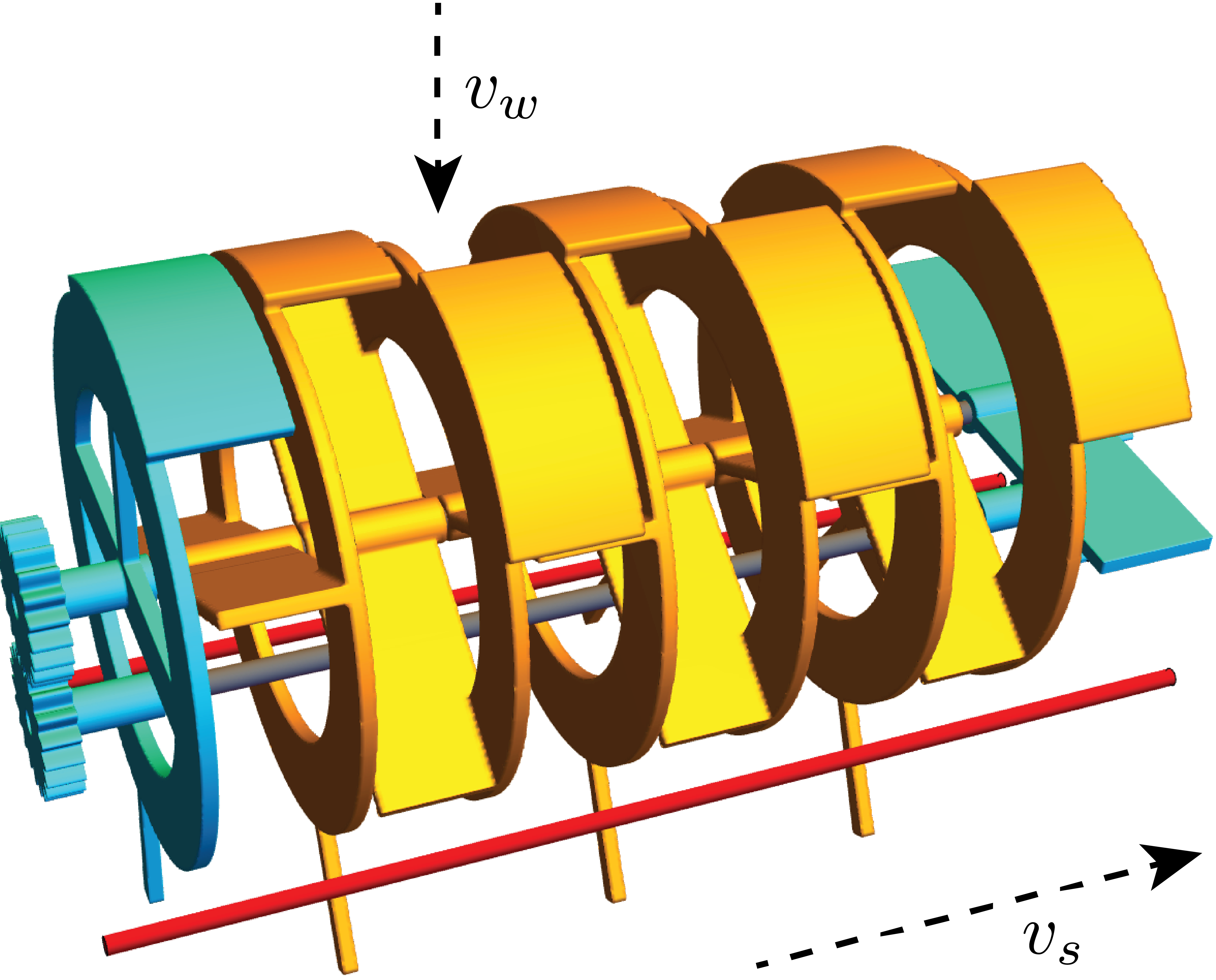
3D printed final design after a decade of development. Wind blows down, solitons move right. Deflector of one element selectively shields the wing of the next, causing wind torque to rotate the next’s tail to the opposite (red) stopping rod. Periodic boundary element, shown in motion, is split into two (cyan) pieces connected coaxially via (gray) rod and (cyan) gears.
REFERENCES (* indicates undergraduate coauthor)
“Experimental observation of soliton propagation and annihilation in a hydromechanical array of one-way coupled oscillators”, J. F. Lindner, K. M. Patton*, P. M. Odenthal*, J. C. Gallagher*, B. J. Breen, Physical Review E, volume 78, pages 066604(1-5) (2008)
“Electronic and mechanical realizations of one-way coupling in one and two dimensions”, B. J. Breen, A. B. Doud*, J. R. Grimm*, A. H. Tanasse*, S. J. Tanasse*, J F. Lindner, K. J. Maxted*, Physical Review E, volume 83, pages 037601(1-4) (2011)
“A wind-powered one-way bistable medium with parity effects”, T. Rosenberger*, G. Schattgen*, M. King-Smith*, P. Shrestha*, K. J. Maxted*, J. F. Lindner, Chaos: An Interdisciplinary Journal of Nonlinear Science, volume 27, pages 023114(1-5) (2017)


Thanks, Mark! I enjoy reading your posts as well.