
Introductory physics often assumes without proof that the drag force on an object is proportional to its velocity, at least for smooth or laminar flow. In particular, a sphere of radius a falling slowly with velocity \underline v in air of viscosity \eta experiences a drag force
\underline{F} = -6\pi \eta a \underline{v},which was first derived by George Stokes in 1851. Here is a digestible derivation of the force on an idealized sphere in an upward flowing fluid using Mathematica, including motivation for the underlying Navier-Stokes fluid-flow equations.
Vectors (with singly-indexed components that can be arranged in column matrices) are underlined while second-rank tensors (with doubly-indexed components that can be arranged in square matrices) are doubly-underlined.
Navier-Stokes Equations
Stress tensor
Recall that pressure perpendicular to the x-direction due to force in the x-direction is
p_x = \frac{dF_x}{da_x},and the shear perpendicular to the y-direction due to velocity changes in the x-direction is
\tau_{xy} = \frac{dF_x}{da_y} = \eta \frac{dv_x}{dy},where \eta = \mu is the dynamic viscosity. For an isotropic fluid, symmetrize this to
\underline{\underline{\tau}} = \eta\left( \underline{\nabla}\,\underline{v} + (\underline{\nabla}\,\underline{v})^T \right)= \eta\left( \underline{\nabla}\,\underline{v} + \underline{v} \,\underline{\nabla} ) \right),where the pressure and the shear combine to form the stress tensor
\underline{\underline{\sigma}} = -p \underline{\underline{I}}+\underline{\underline{\tau}},so the force
\underline{F} = \oiint_{a=\partial V} \hspace{-1.6em} d\underline{a} \cdot \underline{\underline{\sigma}} = \iiint_V \hspace{-0.4em} dV\, \underline{\nabla} \cdot\underline{\underline{\sigma}} = \iiint_V \hspace{-0.4em} dV\, \underline{f}.Continuity Equation
The time rate of change of the fluid density \rho is minus the divergence of the mass current \underline{J} = \rho \underline{v},
\partial_t \rho = -\underline{\nabla} \cdot \underline{J},which for constant density simplifies to a divergence-less velocity field
0 = \underline{\nabla} \cdot \underline{v}.Newton’s Second Law
For an infinitesimal fluid element of velocity \vec v(t, \vec r), the force per unit volume
\rho\left( \partial_t\underline{v}+\underline{v}\cdot \underline{\nabla}\, \underline{v} \right)= \rho \frac{d\underline{v}}{dt} = \underline{f} = \underline{\nabla} \cdot \underline{\underline{\sigma}}.For a stationary flow, so \partial_t\underline{v} = \underline{0}, and slow fluid, so terms \mathcal{O}(v^2) are negligible, this reduces to
\begin{aligned}\underline{0} &= \underline{\nabla} \cdot \underline{\underline{\sigma}} \\ &= -\underline{\nabla}\,p + \underline{\nabla}\cdot \underline{\underline{\tau}} \\ &= -\underline{\nabla}\,p + \eta \left(\underline{\nabla} \cdot \underline{\nabla}\,\underline{v} + \underline{\nabla} \cdot \underline{v}\, \underline{\nabla} \right) \\ &= -\underline{\nabla}\, p + \eta \Delta \underline{v},\end{aligned}where the Laplacian \underline{\nabla} \cdot \underline{\nabla} = \nabla^2 = \Delta. Hence, the relevant Navier-Stokes equations
\boxed{\begin{array}{ccc}\underline{\nabla}\,p & = & \eta \Delta \underline{v}, & (1)\\ \underline{\nabla}\cdot \underline{v} & = & 0, & (2) \end{array}}plus boundary conditions determine the fluid pressure p and velocity \underline{v}.
Pressure and Velocity
Although the computation can be done by hand (as Stokes did), Mathematica eases the workload.
Coordinates
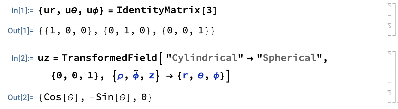
Due to the sphere, introduce spherical coordinates \{r, \theta,\phi \} with unit vectors \{\underline{u}_r, \underline{u}_\theta, \underline{u}_\phi \}, and due to the distant uniform flow, introduce the cylindrical unit vector \underline{u}_z.
Solve Eq. (1) for Velocity
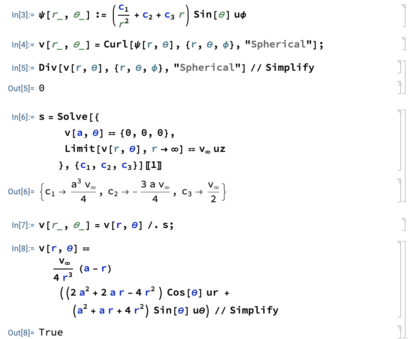
Because the divergence of any curl vanishes, take the fluid velocity (with respect to the sphere) to be the curl of a vector field \underline{v} = \underline{\nabla} \times \underline{\psi}, where the educated guess
\underline{\psi}(r,\theta) = \underline{u}_\theta \left( \frac{c_1}{r^2}+c_2 + c_3 r \right) \sin\theta,subject to the sticky boundary at the sphere and the uniform boundary at infinity, implies
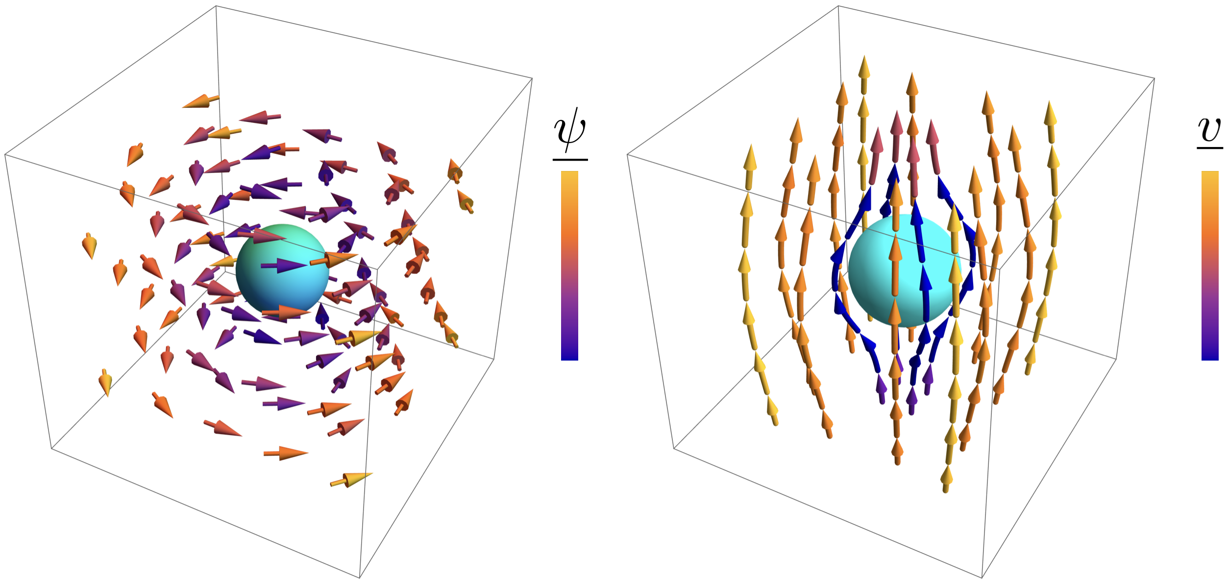
\begin{aligned}\underline{v}(r,\theta) = \frac{v_\infty}{4r^3}(a-r)\big((&\underline{u}_r(2a^2+2ar-4r^2)\cos\theta \\ &+\underline{u}_\theta (a^2+ar+4r^2)\sin\theta\big).\end{aligned}
\underline{\psi}(r,\theta) mainly swirls about the vertical so that its curl \underline{v}(r,\theta) mainly streams upward.
Shear
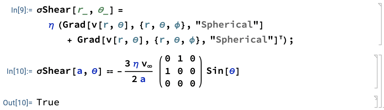
From above, the shear is proportional to the symmetrized velocity gradient, and at the sphere’s surface
\underline{\underline{\sigma}}_s(a,\theta) = \underline{\underline{\tau}}(a, \theta) = -\frac{3\eta v_\infty}{2a} \boxed{\begin{array}{ccc}0 & 1 & 0 \\ 1 & 0 & 0 \\ 0 & 0 & 0 \end{array}}\sin\theta.
Solve Eq. (2) for Pressure
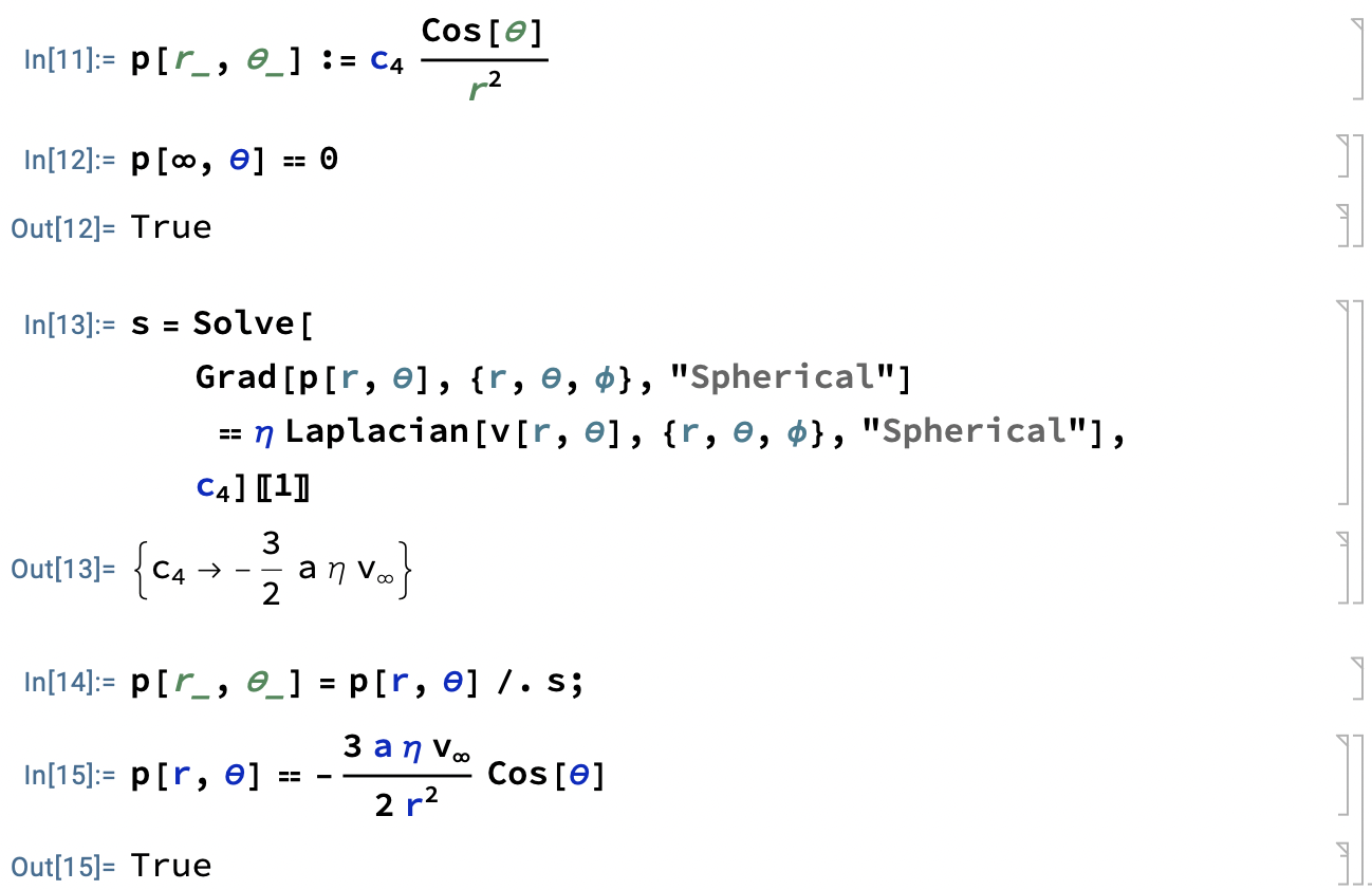
As another educated guess (as they are easy to check with Mathematica), take the pressure (relative to atmospheric pressure) to be of the form
p(r,\theta)= c_4 \frac{\cos\theta}{r^2},which satisfies the boundary condition p(\infty,\theta) =0 . Substituting into the Navier-Stokes pressure equation fixes the constant, so
p(r,\theta)= -\frac{3 \eta a v_\infty}{2r^2} \cos\theta.
The corresponding pressure stress at the sphere’s surface
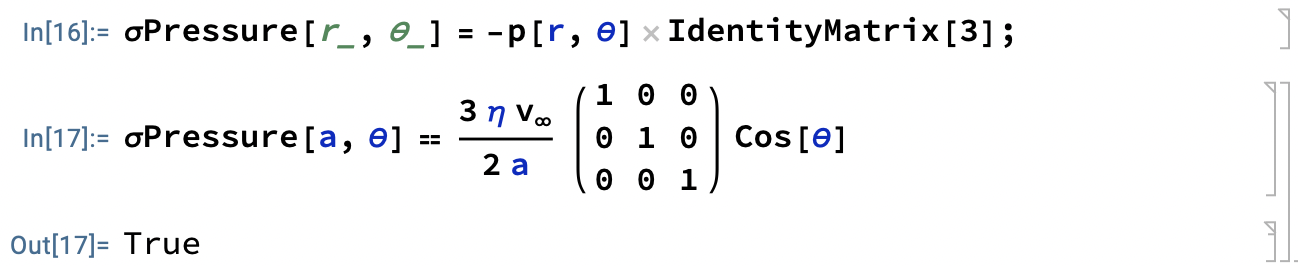
\underline{\underline{\sigma}}_p(a, \theta) = -p(a, \theta)\underline{\underline{I}} = \frac{3\eta v_\infty}{2a} \boxed{\begin{array}{ccc}1 & 0 & 0 \\ 0 & 1 & 0 \\ 0 & 0 & 1 \end{array}}\cos\theta.
Force
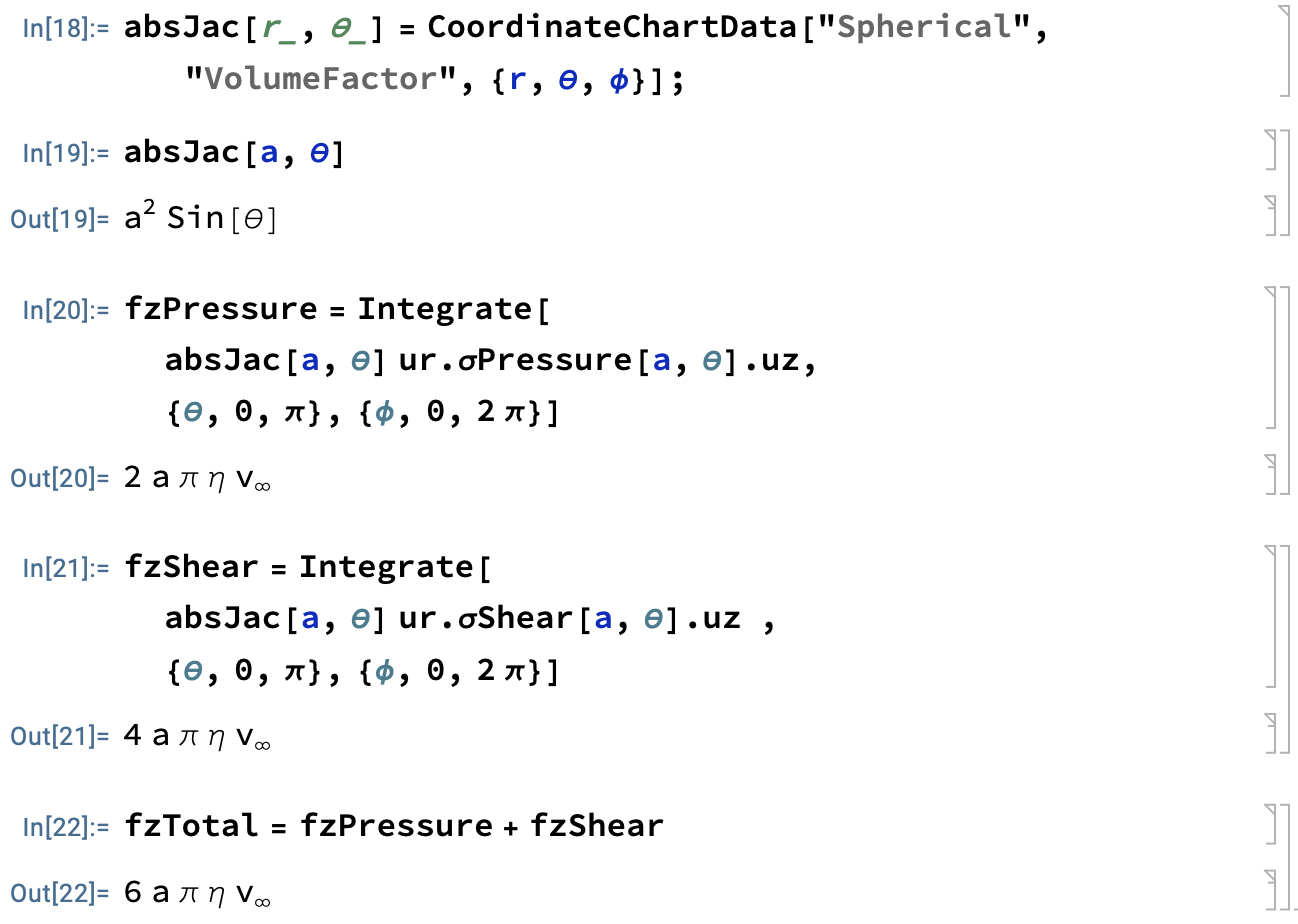
The radial pressure on the sphere in the \underline{u}_z direction is
\begin{aligned}F_p &= \oiint_{S} dS\, \underline{u}_r \cdot\underline{\underline{\sigma}}_p(a,\theta)\cdot\underline{u}_z \\ &= \int_0^\pi\hspace{-0.5em}d\theta \int_0^{2\pi}\hspace{-1em}d\phi \left(a^2 \sin\theta\right) \frac{3 \eta v_\infty}{2a} \cos^2\theta \, \\&= 2 \pi \eta a v_\infty,\end{aligned}and the radial shear on the sphere in the \underline{u}_z direction is
\begin{aligned}F_s &= \oiint_{S} dS\, \underline{u}_r \cdot\underline{\underline{\sigma}}_s(a,\theta)\cdot\underline{u}_z \\ &= \int_0^\pi\hspace{-0.5em}d\theta \int_0^{2\pi}\hspace{-1em}d\phi \left(a^2 \sin\theta\right) \frac{3 \eta v_\infty}{2a} \sin^2\theta \, \\&= 4 \pi \eta a v_\infty = 2F_p,\end{aligned}so the total upward force magnitude
\begin{aligned}F = F_p + F_s = 6 \pi \eta a v_\infty.\end{aligned}
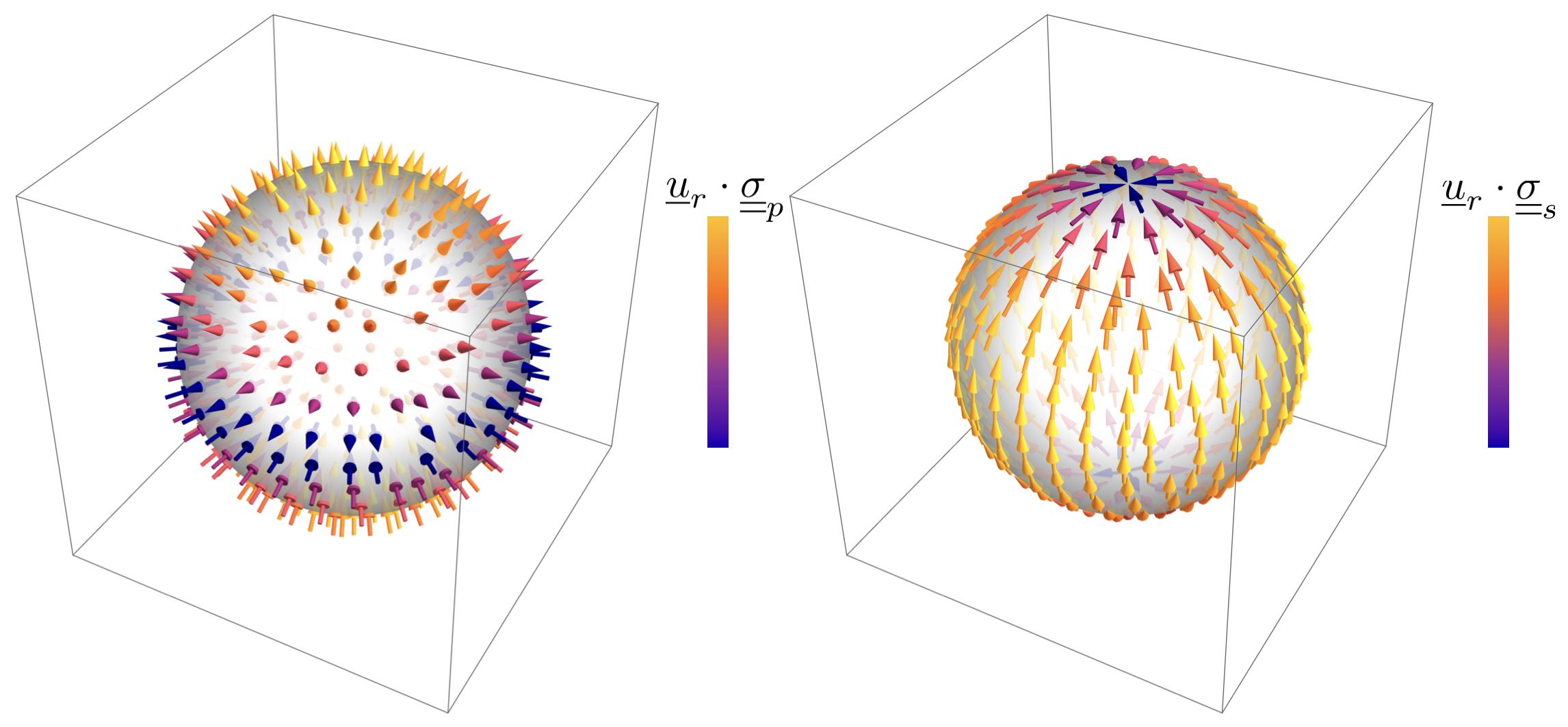
The pressure “blows” from the bottom and “sucks” from the top, but the shear “rubs” twice as hard near the middle!
Thanks, Mark! I enjoy reading your posts as well.