
At my computer Tuesday evening, I receive a message from a university physics chat that is both thrilling and chilling: LIGO + Virgo report a “burst” gravitational wave event, possibly due to a core-collapse supernova (or a binary collision where one object is in the hypothetical “mass gap” between black holes and neutron stars). The burst event is in Orion — near Betelgeuse.
Betelgeuse is a red supergiant star evolving rapidly to an expected supernova. It has dimmed dramatically in recent months, and I’ve seen estimates of thousands to hundreds of thousands of years until it explodes catastrophically in a surge of neutrinos, but 10^{4\pm1} years is so soon astronomically. (In physics, the uncertainty is in the mantissa, but in astrophysics, the uncertainty is in the exponent.)
While a Betelgeuse supernova would irrevocably scar my favorite constellation, it would be the most dramatic astronomical event of my lifetime, outshining Earth’s moon for months before dimming to dark. For a minute or two I seriously contemplate losing Betelgeuse — and gaining a spectacular naked-eye supernova. I frantically search online for more information. Betelgeuse seems safe, but at least one astronomer walks outside to visually check. My breathing returns to normal. More time to prepare the next generation neutrino detectors.
Enjoy Orion while you can, because sometime soon, Betelgeuse is gonna blow.
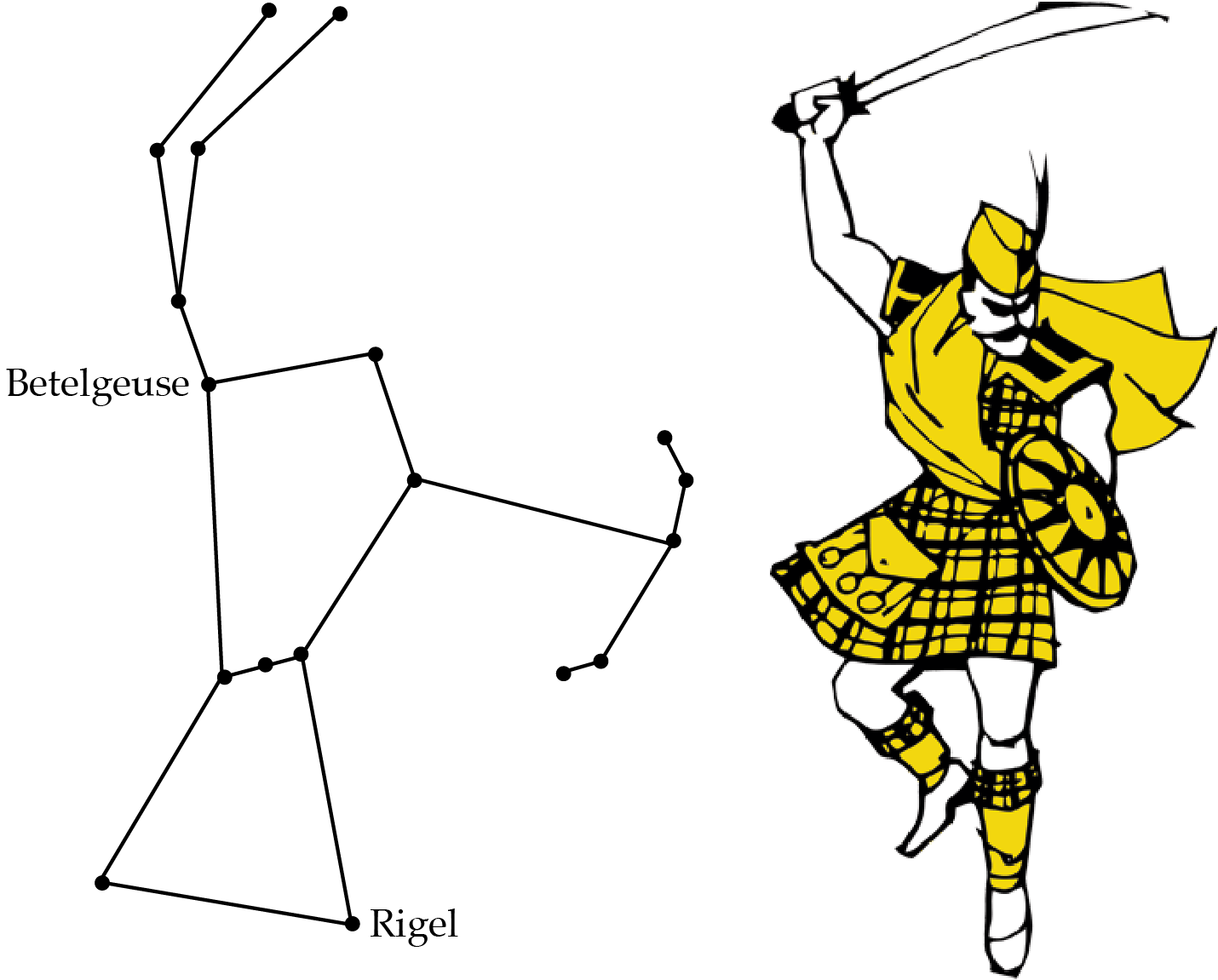
A Betelgeuse supernova would irrevocably damage my favorite constellation, but it would be the most spectacular astronomical event of my lifetime.


Thanks, Mark! I enjoy reading your posts as well.