As a child, I was inspired by Arthur C. Clarke‘s 1956 science fiction novel The City and the Stars to search for patterns in prime numbers. Chapter 6 begins:
Jeserac sat motionless within a whirlpool of numbers. The first thousand primes, expressed in the binary scale that had been used for all arithmetical operations since electronic computers were invented, marched in order before him. Endless ranks of l’s and o’s paraded past, bringing before Jeserac’s eyes the complete sequences of all those numbers that possessed no factors except themselves and unity. There was a mystery about the primes that had always fascinated Man, and they held his imagination still. Jeserac was no mathematician, though sometimes he liked to believe he was. All he could do was to search among the infinite array of primes for special relationships and rules which more talented men might incorporate in general laws. … He knew the laws of distribution that had already been discovered, but always hoped to discover more.

My 95-cent childhood copy of The City and the Stars.
Indeed, I remember manually plotting the smallest primes on graph paper searching for patterns. Today, for example, I know that the prime number theorem describes the asymptotic distribution of the primes, which become less common as they become larger. If \pi(x) is the number of primes less than or equal to x, then \pi(x) \sim x / \log x, for large x.
Here I present an elementary proof of a weak form of the prime number theorem based on a proof by Jan-Hendrik Evertse, which itself was based on work by Paul Erdős.
First recall the binomial theorem
(a+b)^n = \sum_{m=0}^n \binom{n}{m}a^{n-m}b^m,
where the binomial coefficients
\binom{n}{m} = \frac{n!}{m!(n-m)!}.
Also recall the floor function
\lfloor x\rfloor =\max\{n\in \mathbb {Z} \mid n\leq x\},
so
x−1<\lfloor x \rfloor≤x.
Write \log x = \log_e x for the natural logarithm, as is common in pure mathematics and theoretical physics.
Introductory Lemmas
Lemma A: Number of times a prime divides a factorial
\nu_p(n!)=\sum_{m=1}^\infty \left\lfloor \frac{n}{p^m} \right\rfloor
To count the number of times that prime p divides n!, note that each multiple of p\le n contributes a factor of p, each multiple of p^2\le n contributes another factor of p, each multiple of p^3\le n contributes yet another factor of p, and so on, so that
\nu_p(n!) = \left\lfloor \frac{n}{p} \right\rfloor + \left\lfloor \frac{n}{p^2} \right\rfloor + \left\lfloor \frac{n}{p^3} \right\rfloor + \cdots = \sum_{m=1}^\infty \left\lfloor \frac{n}{p^m} \right\rfloor,
where all terms in the sum vanish when p^m > n.
Lemma B: Prime product divides binomial coefficient
0<2b\le a \Rightarrow \prod_{a-b+1\le p\le a} \hspace{-1em}p\hspace{1em} \Bigg| \binom{a}{b}
Since
\binom{a}{b} = \frac{a!}{b!(a-b)!} = \frac{a(a-1)\cdots (a-b-1)}{b(b-1) \cdots \hspace{2.1em} 1\hspace{2.1em}},
each prime b<b+1\le a-b+1\le p\le a divides the numerator but not the denominator, and thus so does their product.
Lemma C: Prime power divides binomial coefficient
a > b > 0,\ p^m\Big| \binom{a}{b}\ \Rightarrow\ p^m \le a
By Lemma A, the number of times a prime divides a binomial coefficient
\begin{aligned}\nu_p\left(\binom{a}{b}\right)&=\nu_p\left(\frac{a!}{b!(a-b)!}\right)\\ &= \sum_{m=1}^\infty \left( \left\lfloor \frac{a}{p^m} \right\rfloor-\left\lfloor \frac{a-b}{p^m} \right\rfloor-\left\lfloor \frac{b}{p^m} \right\rfloor \right).\end{aligned}
Each positive integer summand
\begin{aligned}&\left\lfloor \frac{a}{p^m} \right\rfloor-\left\lfloor \frac{a-b}{p^m} \right\rfloor-\left\lfloor \frac{b}{p^m} \right\rfloor \\& < \frac{a}{p^m}-\left( \frac{a-b}{p^m}-1 \right)-\left( \frac{b}{p^m}-1\right)=2,\end{aligned}
and so must be either 0 or 1. Furthermore, since each summand with p^m>a>b is 0, the sum can grow no larger than the largest m for which p^m \le a.
Lemma D: Bounds on the symmetric binomial coefficient
n\in\mathbb{N}_1\ \Rightarrow\ \frac{2^n}{n+1} \le \binom{n}{\lfloor n /2 \rfloor }\le 2^{n-1}
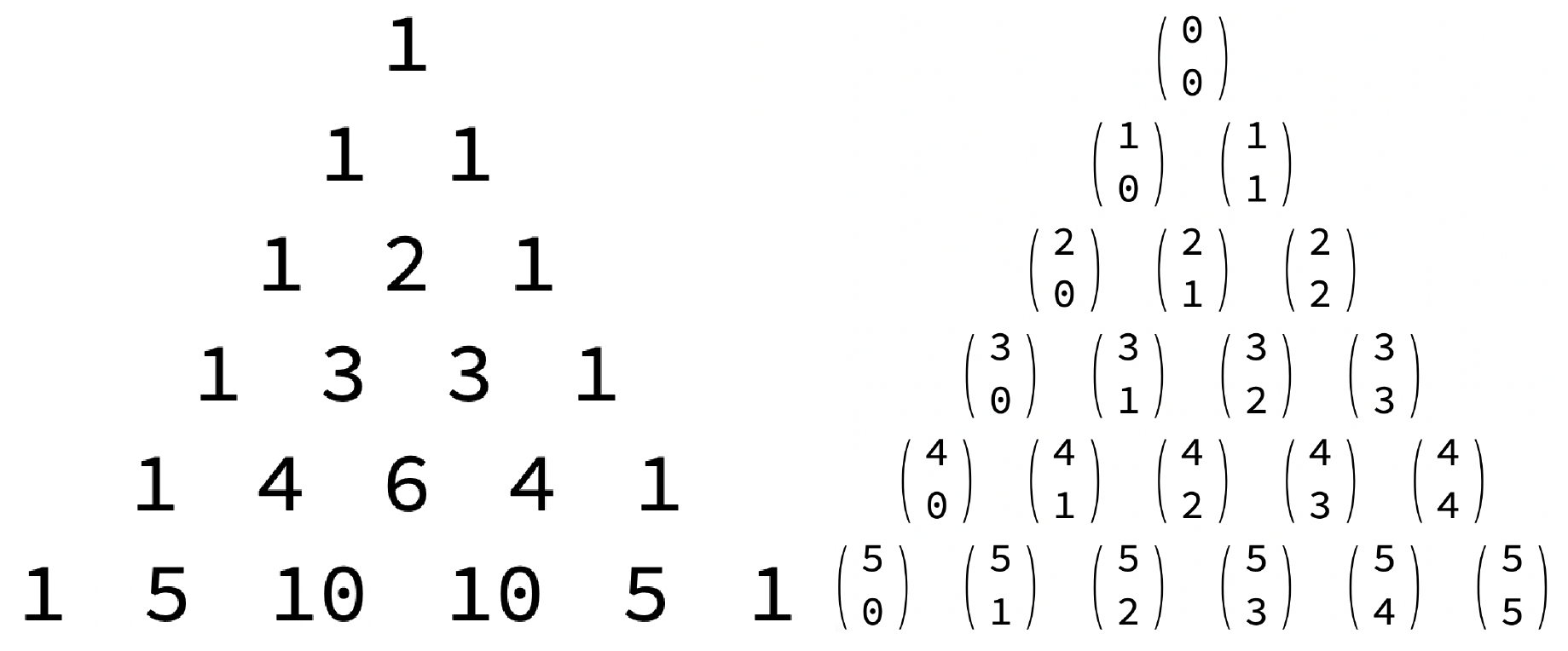
For the lower bound, since the central binomial coefficient (corresponding to the middles of the rows of Pascal’s triangle) is largest,
2^n=(1+1)^n=\sum_{m=0}^n\binom{n}{m}1^m 1^{n-m}\le(n+1) \binom{n}{\lfloor n/2 \rfloor}.
For the upper bound, first let n=2k+1 be odd, so
\binom{2k+1}{k}=\binom{2k+1}{k+1}
and
\begin{aligned}\binom{n}{\lfloor n/2 \rfloor} &=\binom{2k+1}{k}=\frac{1}{2}\left( \binom{2k+1}{k}+\binom{2k+1}{k+1} \right) \\& \le \frac{1}{2}\sum_{m=0}^{2k+1} \binom{2k+1}{m}=(1+1)^{2k}=2^{2k}=2^{n-1}.\end{aligned}
Next let n=2k be even, so
\binom{2k}{k-1}=\binom{2k}{k+1}=\binom{2k}{k}\frac{k}{k+1}\ge \frac{1}{2}\binom{2k}{k}
and
\begin{aligned}\binom{n}{\lfloor n/2 \rfloor} &=\binom{2k}{k}\le\frac{1}{2}\left( \binom{2k}{k-1}+\binom{2k}{k}+\binom{2k}{k+1} \right) \\& \le \frac{1}{2}\sum_{m=0}^{2k} \binom{2k}{m}=(1+1)^{2k-1}=2^{2k-1}=2^{n-1}.\end{aligned}
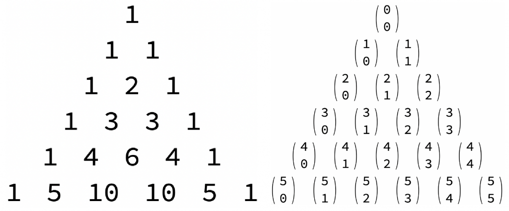
Pascal’s triangle and binomial coefficients.
Theorem
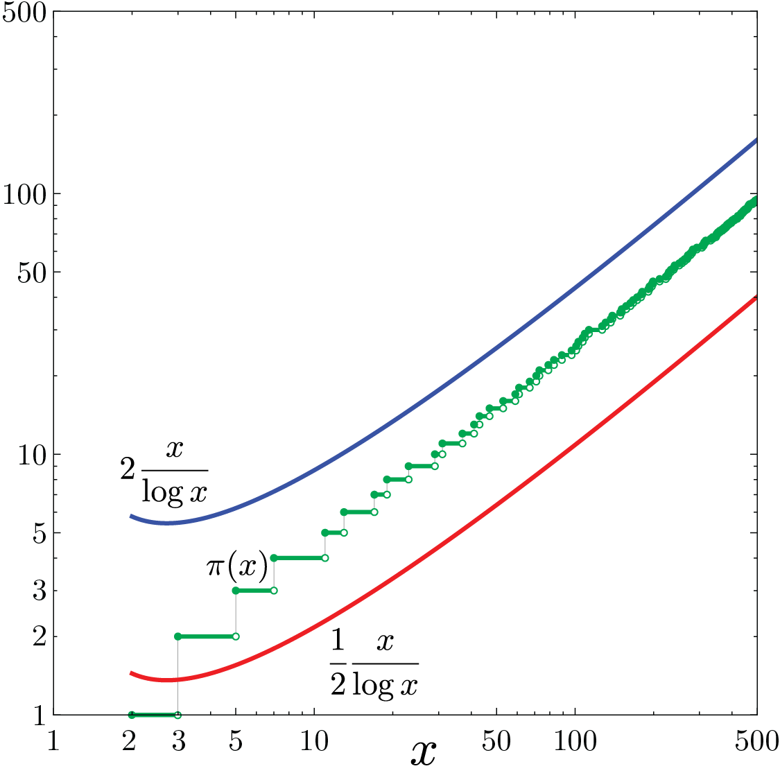
The number of primes less than or equal to x\ge 3 is bounded above and below by multiples of x/\log x, specifically
\frac{1}{2} \frac{x}{\log x} \le \pi(x) \le 2 \frac{x}{\log x}.
Equivalently, in Donald Knuth‘s notation, \pi(x) = \Theta(x / \log x), and in G. H. Hardy‘s notation, \pi(x) \asymp x/\log x. (The stronger relation \pi(x) \sim x / \log x is harder to prove.)
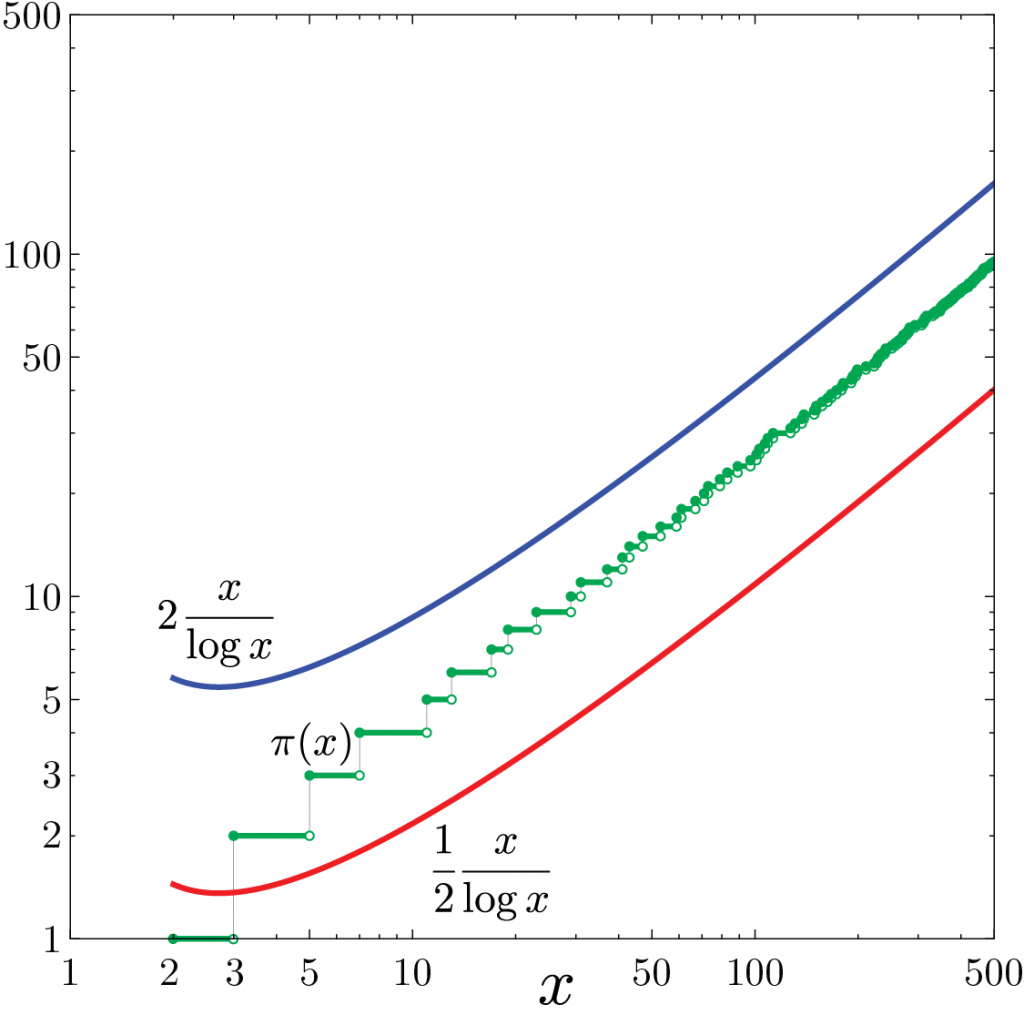
Bounding the prime counting function.
By direct calculation, both bounds are good for 3\le x\le 500, as in the above graph. Let n=\lfloor x \rfloor, so n\le x < n+1.
Lower bound
Prime factor the central binomial coefficient
\binom{n}{\lfloor n/2 \rfloor} = p_1^{k_1}\cdots p_t^{k_t}.
By Lemma C, 1<p_m \le p_m^{k_m}\le n, and so p_m \le n for m=1, \ldots,t. Thus the number of prime factors t \le \pi(n), which combined with Lemma D gives
\frac{2^n}{n+1} \le \binom{n}{\lfloor n/2 \rfloor} \le n^{\pi(n)},
and so
\begin{aligned}\pi(x)&=\pi(n)\ge \frac{n \log 2-\log(n+1)}{\log n}\\ & \ge \frac{(x-1)\log 2-\log(x+1)}{\log x}\\ & \ge \frac{1}{2}\frac{x}{\log x},\end{aligned}
where the final inequality is by Appendix Lemma E.
Upper bound
Proceed by induction. If n=2m+1 is odd, then by Lemma D and B,
2^{2m} \ge \binom{2m+1}{m}\ge \prod_{m+2\le p \le 2m+1} \hspace{-1.8em}p\hspace{0.8em} \ge (m+2)^{\pi(2m+1)-\pi(m+1)},
and so
\pi(2m+1)-\pi(m+1)\le \frac{2m \log 2}{\log(m+2)}.
Use the induction hypothesis on \pi(m+1) with m+2>m+1>n/2 to find
\begin{aligned}\pi(n)=\pi(2m+1)&=\frac{2m \log 2}{\log(m+2)}+\pi(m+1) \\ &\le \frac{2m \log 2}{\log(m+2)}+2\frac{m+1}{\log(m+1)} \\ & < \frac{2m\log 2 + 2m+2+\log 2}{\log(m+1)}\\ & < \frac{n(\log 2 + 1)+1}{\log(n/2)}\\ & < 2\frac{n}{\log n},\end{aligned}
where the final inequality is by Appendix Lemma F. If n is even, then n-1 is odd and
\pi(n)=\pi(n-1)\le 2\frac{n-1}{\log(n-1)}<2\frac{n}{\log n},
as x/\log x is increasing for x>e .
Appendix Lemmas
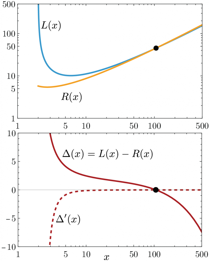
Lemma E: For lower bound
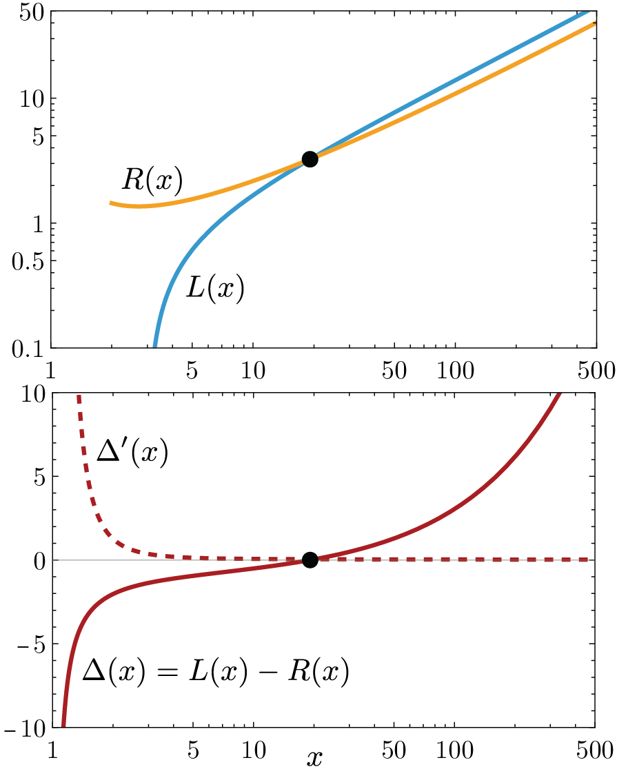
L(x)=\frac{(x-1)\log 2-\log(x+1)}{\log x}\ge \frac{1}{2}\frac{x}{\log x}=R(x)\Leftarrow x>100

The left and right functions don’t intersect after x ≈ 19.1.
If the difference
\Delta(x) = L(x)-R(x),
then the derivative
\Delta^\prime(x) = N(x)/D(x),
where
N=N_0+N_1 x+N_2 x^2,
and
\begin{aligned}N_0 &= 2 \log 2 + 2\log(1+x)\\&>0 \Leftarrow x>-1/2,\\ N_1 &=1-3\log x+ 2\log 2\log x+2\log(1+x) \\ &> 1-3\log x+2\log 2\log x + 2\log x \\&= 1+(2\log 2-1)\log x\\&>(2\log 2-1)\log x\\&> 0 \Leftarrow x>1, \\N_2 &= 1-2\log 2-\log x + 2\log 2\log x\\&= (1-2\log 2)(1-\log x)\\&>0 \Leftarrow x>e,\\D& =2x(1+x)(\log x)^2\\&>0\Leftarrow x>1.\end{aligned}
Hence, \Delta'(x) >0 for x>e, L(x) and R(x) continue separating after crossing at x\approx 19.1, and the lemma follows.
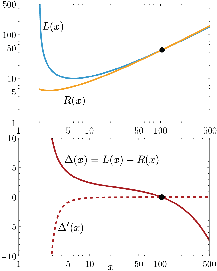
Lemma F: For upper bound
L(x)= \frac{n(\log 2 + 1)+1}{\log(n/2)} < 2\frac{n}{\log n}=R(x)\Leftarrow x>500
The left and right functions don’t intersect after x ≈ 106.
If the difference
\Delta(x) = L(x)-R(x),
then the derivative
\Delta^\prime(x) = N(x)/D(x),
where
N=N_0+N_2 (\log x)^2,
and
N_0=2\log 2(m_0\log x+b_0)x <0 \Leftrightarrow
\log x > -\frac{b_0}{m_0}\Leftrightarrow x > \exp\left(-\frac{b_0}{m_0}\right) \Leftrightarrow
x > \exp\left(\frac{1}{1+2/\log 2}\right)\approx 1.29,
N_2=-1+(m_2\log x+b_2)x < 0 \Leftarrow
\log x > -\frac{b_2}{m_2}=-\frac{1+2\log 2-(\log 2)^2}{\log 2-1} \Leftrightarrow
x >\exp\left(\log 2-1-\frac{2}{\log 2-1}\right)\approx 498,
and
D=x(\log x)^2(\log x-\log 2)^2>0 \Leftarrow x>2.
Hence, generously, \Delta'(x) <0 for x>500, L(x) and R(x) continue separating after crossing at x\approx 106, and the lemma follows.


Thanks, Mark! I enjoy reading your posts as well.