Ancient cultures everywhere observed seven “wanderers” move against the apparently fixed stars of the night sky: our star the sun, our natural satellite the moon, and the brightest planets Mars, Mercury, Jupiter, Venus, and Saturn. In many languages, these wanderers became the basis for the names of the seven days of the week; for example, in English & French the days are:
A falling cat’s twisting returns its shape to normal but rotates its body to land feet down. Earth’s spin returns a Foucault pendulum to its initial position in one day but rotates its oscillation plane. Parallel parking cyclically rotates a car’s front wheels but shifts the car sideways. These are examples of nonholonomic motions or mechanical anholonomies.
Hwan Bae, Norah Ali, and I just published a featured article in the journal Chaos on another famous anholonomy, Hannay’s hoop, which involves a bead sliding frictionlessly on a horizontal noncircular hoop: A slow cyclic rotation restores the hoop to its original state but unavoidably shifts the moving bead by an angle that depends on the hoop’s geometry. Rotating a noncircular hoop indelibly imprints its geometry on the bead’s motion.
In the limit of slow rotation and fast beads, the shift is called Hannay’s angle (and is analogous to Berry’s phase in quantum mechanics). We mathematically generalized the shift to any speed, fast or slow, and were able to observe it in a simple experiment involving wet ice cylinders sliding in 3D printed channels.
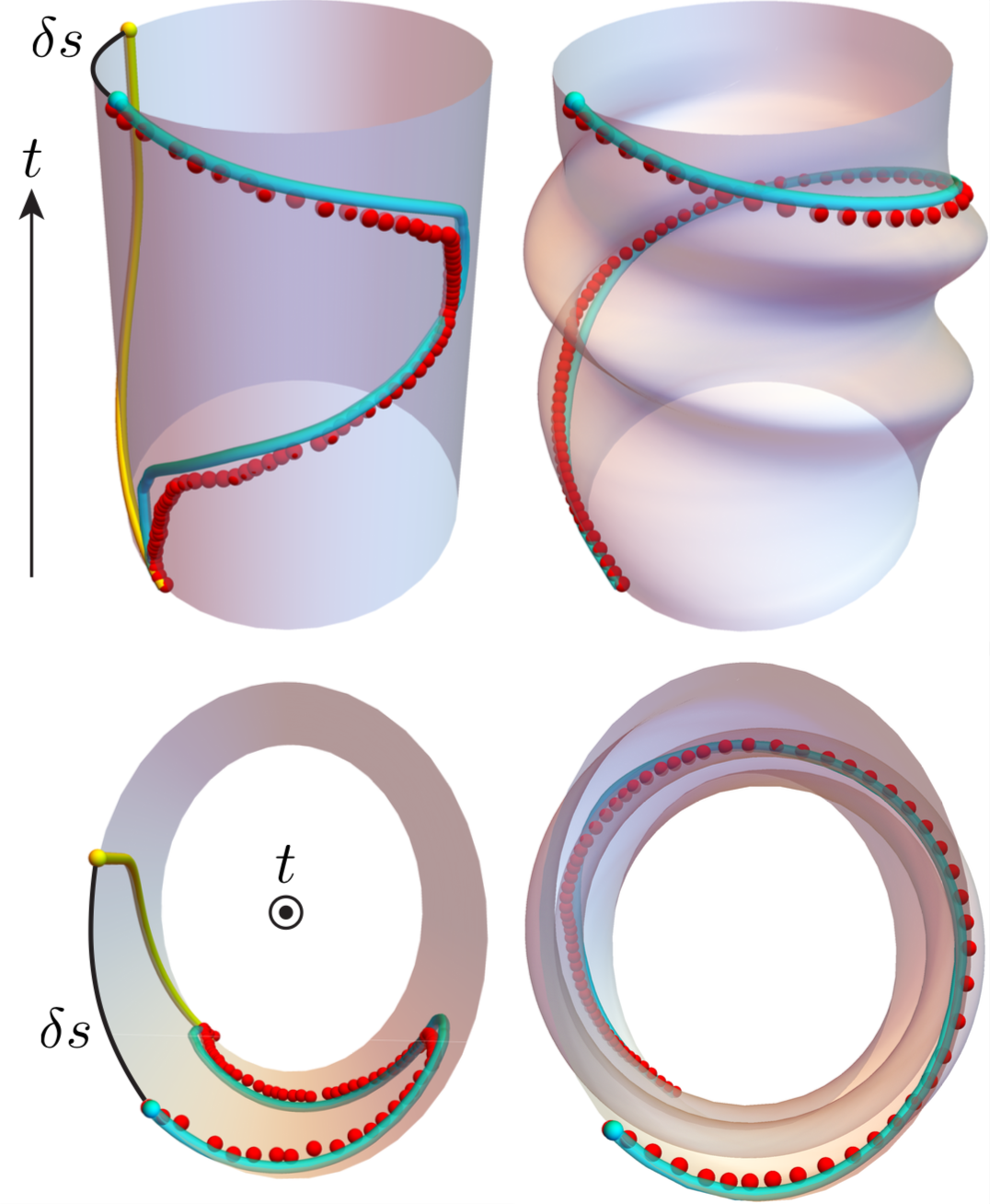
Spacetime diagrams of a bead sliding on spinning hoop in the hoop (left) and lab (right) frames. Red spheres are experiment, cyan tubes are simulation, yellow tubes numerically extrapolates bead sliding in the absence of hoop spinning, and black arcs are the generalized Hannay’s shift.
Norton’s Dome is a fascinating counterexample in classical mechanics: A frictionless mass balanced at the dome’s top can remain there forever — but can also spontaneously slide down!
A mass slides down Norton’s dome from rest and then is kicked back up to rest.
The Shape
Norton’s dome has a cubed square root profile: if the downward height is z at dome arc lengths, then
\frac{z}{z_m} = \left(\frac{s}{s_m}\right)^{3/2}.
f max height z_m = 2/3 when max arc length s_m = 1, then
z = \frac{2}{3}s^{3/2}.
By the Pythagorean theorem, ds^2 = dx^2 + dz^2, and so
The acceleration along the dome increases as the square root of the arc length. Combine the equation of motion with the initial conditions s[0]=0 and \dot{s}[0]=0, corresponding to a mass at rest on top of the dome, to form an initial value problem (IVP).
The Solutions
Surprisingly, two solutions exist: infinite rest
s[t] = 0
and spontaneous sliding
s[t] = \frac{1}{144} t^4.
To check the latter, differentiate to get
\dot s = \frac{1}{36} t^3, \ddot s = \frac{1}{12} t^2 = \sqrt{s}.
How can a physical system have two evolutions?
The Resolution
If an IVP’s equations are continuous, solutions exist; if the first derivatives are also continuous, the solution is unique. In this case, the square root \sqrt{s} in the equation of motion means that the first derivative is not continuous at the origin, so solutions exist but are not unique.
The peak of Norton’s Dome is continuous, and its slope is continuous, but the slope of its slope is discontinuous. The apex of a cone is more extreme, as its slope is discontinuous.
All I can think of to describe my experience in the Standard model’s 50th anniversary conference is to repeatedly yell the word wow, until I have lost the will to do so. I am at a loss of words, but I will attempt to put my flustered speech in perspective.
Imagine Albert Einstein dedicating some of his time to share his findings with you. One of the greatest minds explaining the greatest discoveries to you. Not to get greedy but imagine all the great minds of a generation dedicating a couple of days to do just that. I am of course referring to 1927 fifth Solvay International Conference featuring the most prominent names in physics; names including Albert Einstein, Niels Bohr, Paul Dirac, Erwin Schrodinger, and Wooster’s very own Arthur Compton. Attending a conference of such magnitude is a dream for any aspiring physicist, and this is how it felt to be a part of the Standard Model Conference.
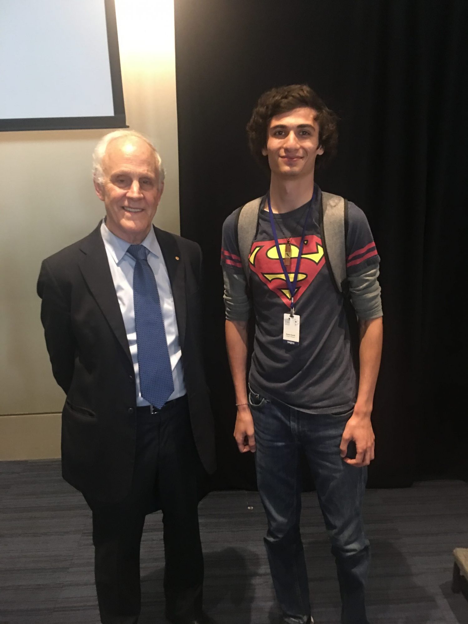
Dr. David Gross and Haidar Essili during SM@50.
Dr. Gerard ‘t Hooft and Haidar Essili during SM@50.
In this conference, I listened to my idols talk about the successes of this field I aspire to be a part of. I also listened to my idols talk of the short comings of this theory. No where is the Greek quote “the more I know, the more I know I know nothing” more true than when the most knowledgeable scientists in a field tell of how little we know. In fact, the Standard Model, often dubbed the Theory of Almost Everything, accounts for a mere 4% of the universe’s constituents and even that we don’t fully understand. I sat in the back when speakers took turns calling upon the back rows of undergraduates for help in advancing this theory in the future. Imagine Einstein passing the torch to you. Imagine Einstein asserting the back rows will certainly produce the next Nobel Laureate. Wow!!”
Gerard t’ Hooft (1999) asks Steven Weinberg (1979) a question after the final talk at SM@50. Carlo Rubbia (1984) and David Gross (2004) listening (center left part of the lecture room). In Front of us were Jerome Friedman (1990) and George Smoot (2006). Samuel C.C. Ting (1976) and Takaaki Kajita (2015) left after their presentations during the weekend. In parenthesis are the years of their Nobel Prize in Physics award.
Spring is a big time for outreach here at Wooster Physics. The Physics Club runs demonstrations for local elementary schools, doing often two outreach visits a week during the spring. (In the fall, we are usually prepping for this flurry of events — sending letters to the schools and doing scheduling, and training new students on the outreach activities.)
We also have two big events on campus. The Physics Club runs Science Day, an event for all science clubs on campus to do demos and fun activities for the whole community. And we participate in Expanding Your Horizons, a huge event specifically for middle school girls that incorporates not just women science students and professors from the campus but also professional women from around the community whose job includes an aspect of science.
At Science Day, it’s fun to see what the other sciences on campus are doing. The neuroscience club gets a lot of interest with the brains that they bring.
Brains! Brain hats! Lots of brains!
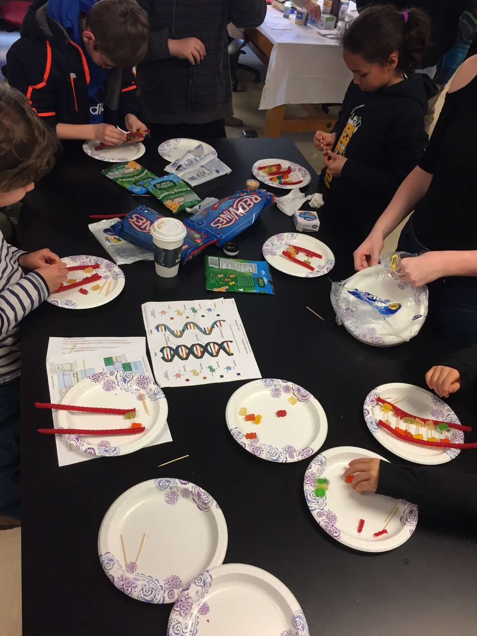
Build your own DNA — so popular, they had to run to the store for more gummy bears
Static charge is awesome!
New this year was a giant size demo from the Astronomy Club to demonstrate how massive objects warp the spacetime around them so that other smaller objects orbit the massive one. This was lots of fun to play with!
Spheres orbiting a massive object warping the fabric of space around it
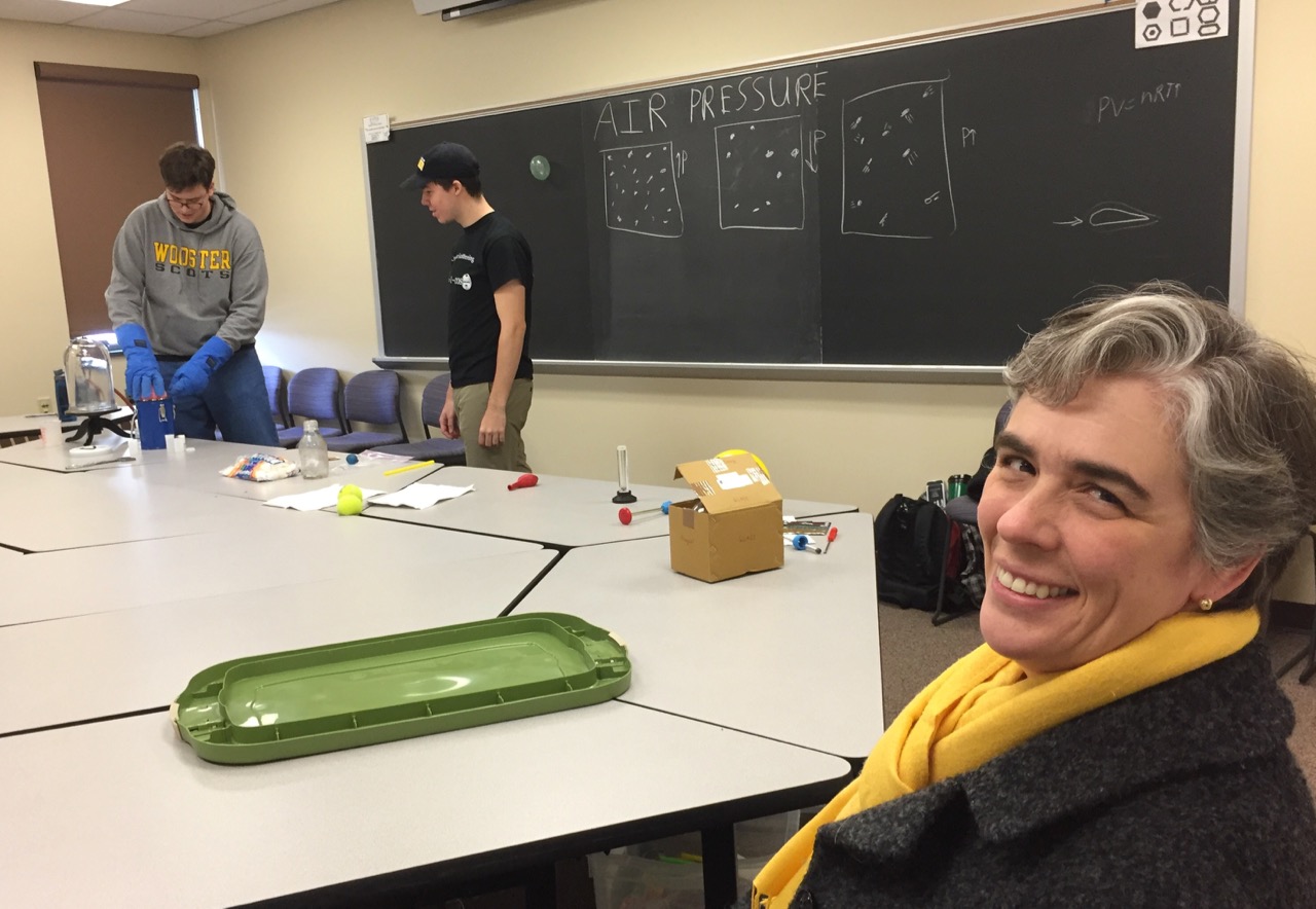
Air pressure is always a favorite, of course, with the liquid nitrogen parts. This year the demo even attracted President Bolton! I think she had a fun morning with lots of physics — it’s probably a good change from administration.
The pink balloon slowly re-inflates as it warms back up to room temperature
President Bolton enjoys a little physics for her spring Saturday.
Bubbling multi-colored lava lamps from chemistry.
Static charge is awesome!
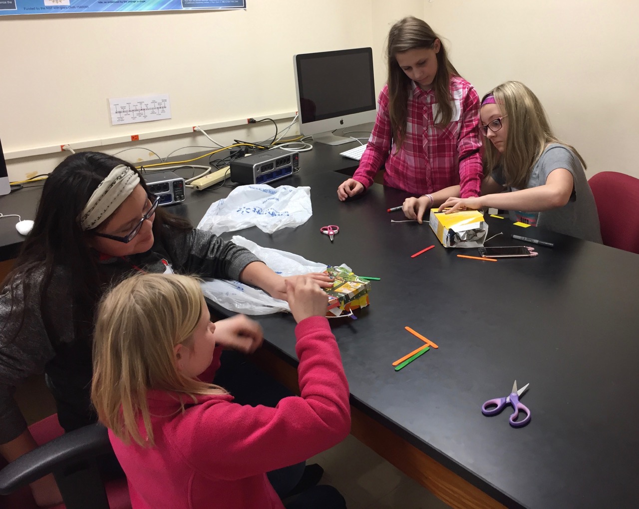
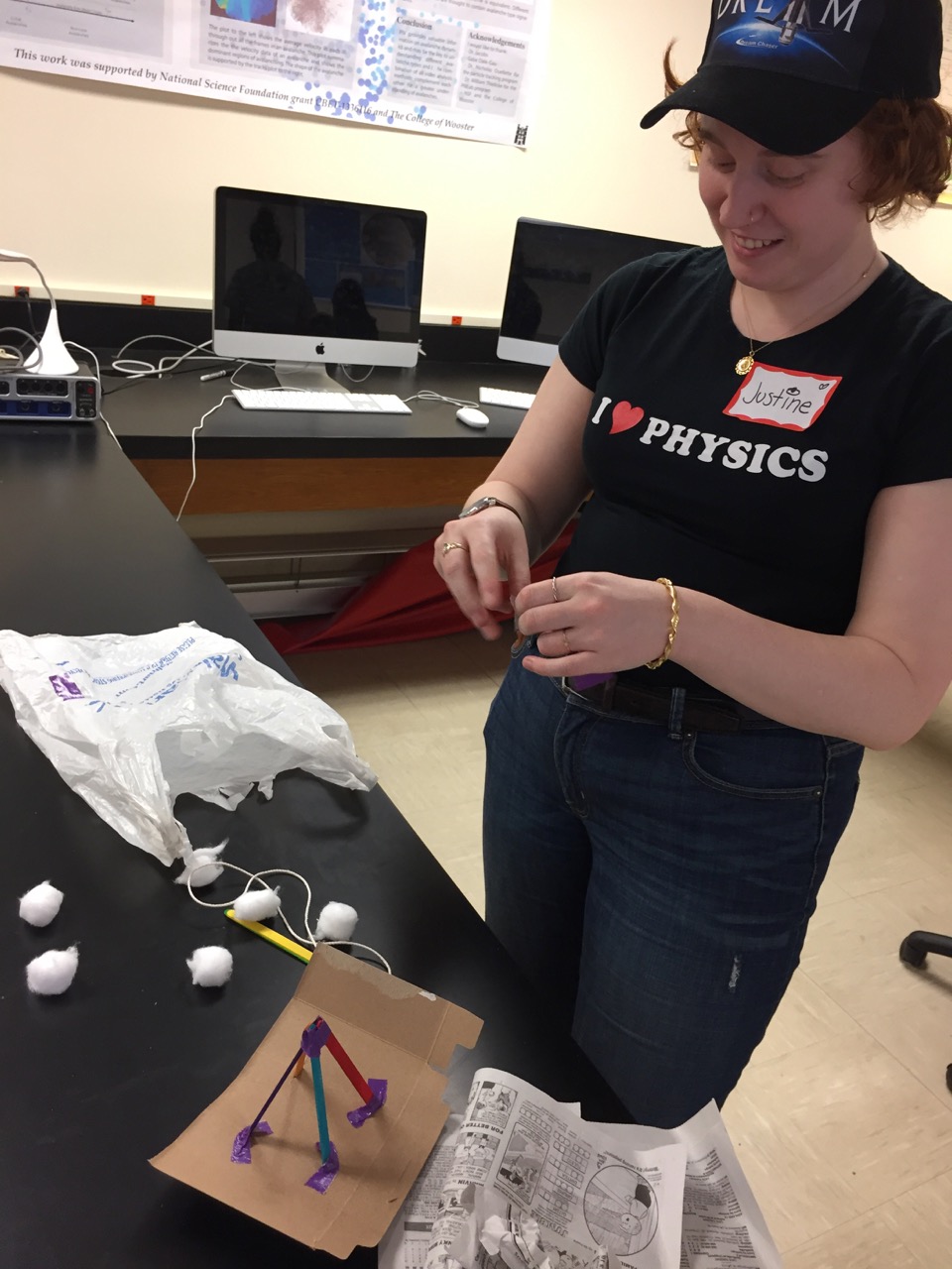
For Expanding Your Horizons, I do the same workshop three times for different groups of girls. We do the “Humpty Dumpty” experiment, where the girls have about 20 minutes with limited materials to create a container to try to protect an egg from breaking during a fall. We drop the eggs from the 3rd floor, so it’s pretty challenging! This year, Dr. DeGroot joined me and we had lots of fun. I love seeing the creativity of the girls — not only in making their containers, but also in decorating and naming their eggs.
Boxes? Cushioning? Parachutes? What else can we try?
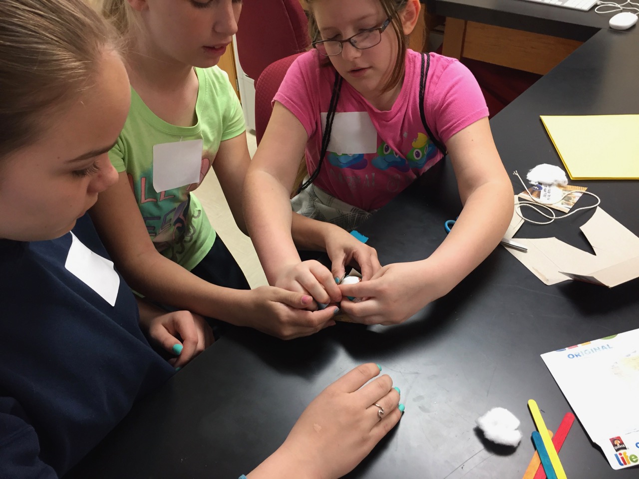
Wrapping the eggs up takes lots of hands and coordination!
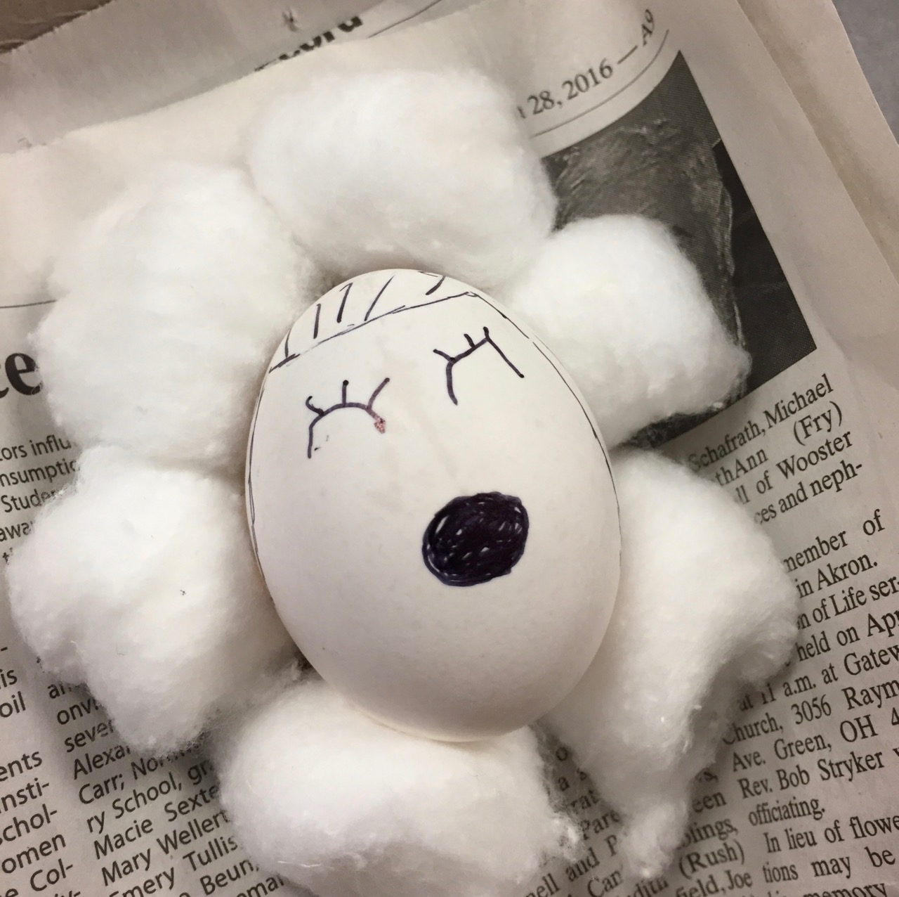
An anxious little egg, waiting in eggs-pectation of the fall.
After helping with the Humpty Dumpty experiment for three years, Justine decided to try it out herself!
And the moment of truth — dropping the eggs from a great height! If the eggs survive, we add them to the Egg Hall of Fame!
The moment of truth — will the eggs survive?
Most of the eggs this year made it! Lesson learned = parachutes really work!
I ran up the stairs to Studio Art. Justine was already rolling out the treadmill, so I climbed another flight of stairs to the old running track and let down both ends of the steel cable, one end connected to the harness and the other to the sandbag counterweight. Our reduced gravity rig was basically a giant Atwood machine leveraging technology perfected recently for flying performers in theatre and cinema. I turned on all the lights in the Crit space, and the wood floor shined.
This Saturday was our last day to work with our dancers before Justine left for LA to present her senior thesis at the March American Physical Society meeting. (From literally thousands of presentations, the APS’s PHYSICS web site would rank Justine’s Moon Dance talk as one of the meeting’s top ten highlights.)
We massed Rachel, and Justine helped her into the harness as I fine-tuned the sandbag mass to simulate lunar gravity. With Rachel sitting expectantly on the floor, Justine and I struggled to raise the sandbag and connect the steel wire to the harness with the carabiners. We moved away, and with an almost surreal lack of effort, Rachel gracefully stood, the sandbag descending as she ascended. I made a mental note to thank Mike for recommending the low-friction pulleys.
Kim and Justine had choreographed treadmill translation sequences for both Kathlyn and Rachel, but the free-dance improvisation proved most successful. Once we got the physics right, I had hoped we would produce something of artistic value, and we had. Our dancers had the grace, and we gave them the power – a superpower.
By approximating lunar and martian gravity for her senior thesis, Justine changed the physics of dance. But her central achievement was the unprecedented and dazzling reduced-gravity performances she elicited from her dancers. Later this century, dancers will dance on Luna and Mars, and Justine has glimpsed that future, and it will be spectacular.
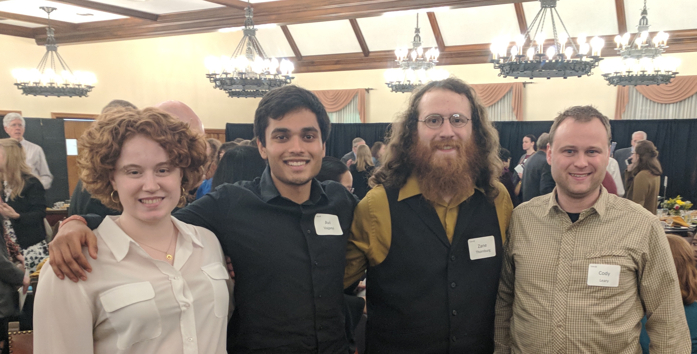
Congratulations class of 2018! I’ve attached a few pictures of some of our seniors and professors who gathered for a quick photo on graduation day (pics courtesy of Zane Thornburg). Special congratulations are in order for Avi Vajpeyi (far left in the second photo), who was selected to be one of the College’s commencement speakers this year!
As my first year as department chair winds up, I am preparing to move to the University of Oregon in Eugene for a one-semester research leave. I’m looking forward to reconnecting with five Wooster physics alumni who are now in the Physics Ph.D. program there!
As I look back on the year, I have a few more random highlights to post that I somehow never found the time to blog about during the busy year!
I enjoyed attending the Senior awards banquet earlier this spring, where Justine Walker, Avi Vajpeyi, and Zane Thorburg (left to right below) were honored for their academic accomplishments. Congrats to all three of you!
The department’s new 3-D printer, housed in Dr. Manz’s Wave Lab, experienced heavy use in multiple research projects, including Collin Hendershot ’18’s project studying the aerodynamics of race car wings of various curvatures. We also used it to 3-D print a plaque honoring Maggie Lankford 16 whose selection as an Apker Award finalist for her I.S. research helped fund the purchase of the printer. Thanks for Jack Mershon ’18 for his help with the plaque!
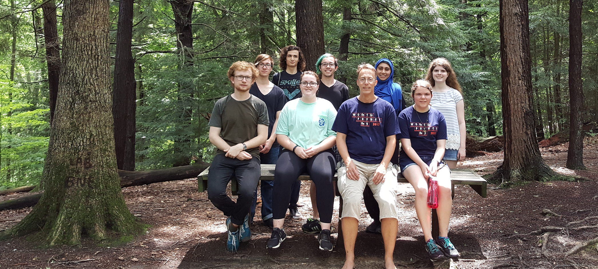
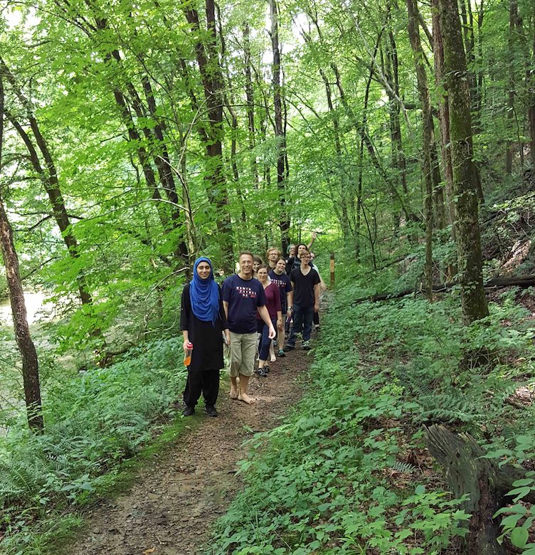
Last summer, students and professors who participated in our NSF-sponsored summer research program paused their work for an afternoon to go on a hike at Wooster Memorial park, a lovely 300 acre wooded area including many miles of trails around a large ravine. I hope this becomes an annual tradition!
The department is looking forward to another exciting summer of research as our 2018 program begins in less than one week! I’ll be sure to blog from Oregon during my leave, so stay tuned.
Mercury has the most noncircular or eccentric orbit of any nondwarf planet in the solar system. This eccentricity has trapped Mercury in a 3:2 spin-orbit resonance, where it rotates three times for every two revolutions. When nearest Sun at perihelion, Sun’s tidal forces are greatest, Mercury’s spin and orbit (or rotation and revolution) nearly match, and Sun momentarily reverses in Mercury’s sky.
For long times, Mercury’s orbit precesses due to the gravity of Jupiter, the oblateness of Sun, and spacetime curvature, first described by Albert Einstein’s theory of General Relativity. For short times, as the animation shows, one solar day lasts two years!
Mercury spins 3 times for every 2 orbits, and 1 day lasts 2 years.
Stationary electric charges generate radial electric fields, and electric fields push positive charges (and pull negative charges). Moving charges also generate circulating magnetic fields, and magnetic fields deflect moving charges perpendicular to both the fields and their motions. All of electromagnetism follows.
In particular, spin a conducting disk in a perpendicular magnetic field, and connect its axle to its circumference using a wire and two sliding contacts, as in the animation. The magnetic field deflects free changes in the disk radially, and they push other charges through the wire. This rotary electric generator converts mechanical motion into electrical current, which can heat the wire and toast bread.
Is the external magnetic field necessary? No! Bend the wire into circles just above and below disk, as in the animation. If the disk spins fast enough, the internal magnetic field of the charges moving in the wire deflects the charges in the disk, which then push the charges through the wire! This dynamo is the closest thing to perpetual motion in classical physics. It generates the magnetic fields of stars and planets, including Earth’s.
Rotary electric generator needs an external magnetic field, but a dynamo generates its own.
The March Meeting is always so exciting — there is so much information here!
Graphene origami and micron-sized laser controlled robots at Marc Miskin’s talk on Tuesday morning. SO COOL!
On Tuesday morning, I went to an outstanding session on Atomic Origami. There is some truly amazing work out there with people designing shapes of graphene (mostly) that fold up on their own into boxes or flowers. Post-doc Marc Miskin gave a really inspiring talk, including showing a little piece of graphene that folds itself up into a triangle only 15 microns on a side — reversibly and repeatedly! Harvard professor David Nelson (who gave a colloquium at Wooster just a few years ago) also gave a wonderfully dynamic talk on criticality and crumpling of paper.
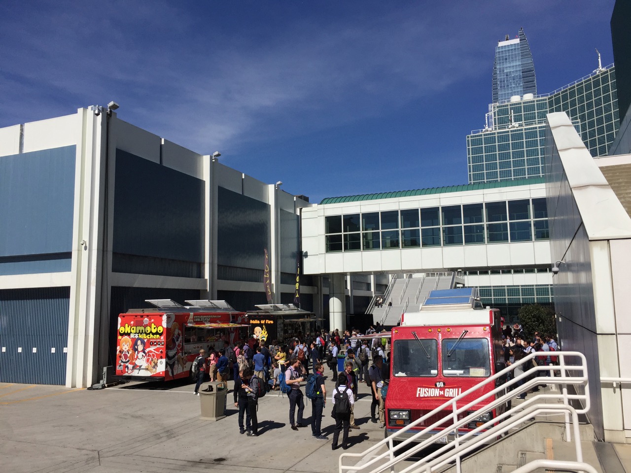
Food trucks and extremely long, slow lines in the sun. Good food though.
Emma Brinton ’18 gave her poster in the afternoon, and got good interest from the crowd.
Meanwhile Justine Walker ’18 and I went to a session on the life and legacy of Millie Dresselhaus. Millie was an absolutely outstanding person and physicist, and the first woman to do so many things. I knew of Millie, of course, but learned so much more about her. I also got to catch up with my Ph.D. advisor Laurie McNeil, who was chairing this session.
Spot the Wooster physicists in the crowd waiting for the graphene superconductivity talk. Hint: look for Michelle’s backpack.
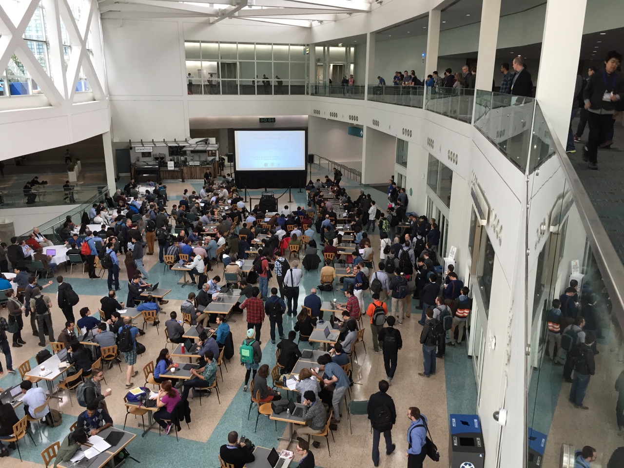
Day 3, Wednesday, started off with a buzz of excitement around an invited talk about graphene and a new discovery of superconductivity. This was actually really interesting since I learned a good bit about graphene and carbon compounds in general the day before at the Millie Dresselhaus session, since she was a tremendous pioneer with carbon (and is known as the Queen of Carbon). I don’t know if everyone was already excited about the talk, but the APS sent out an email basically saying “this talk is so cool we’re projecting it in the cafe”, so then of course everyone came. We had seats at a table, but moved to the balcony when too many people stood in front of us. It was interesting, but I’m not sure if it’s quite the Woodstock of physics event we were hoping for.
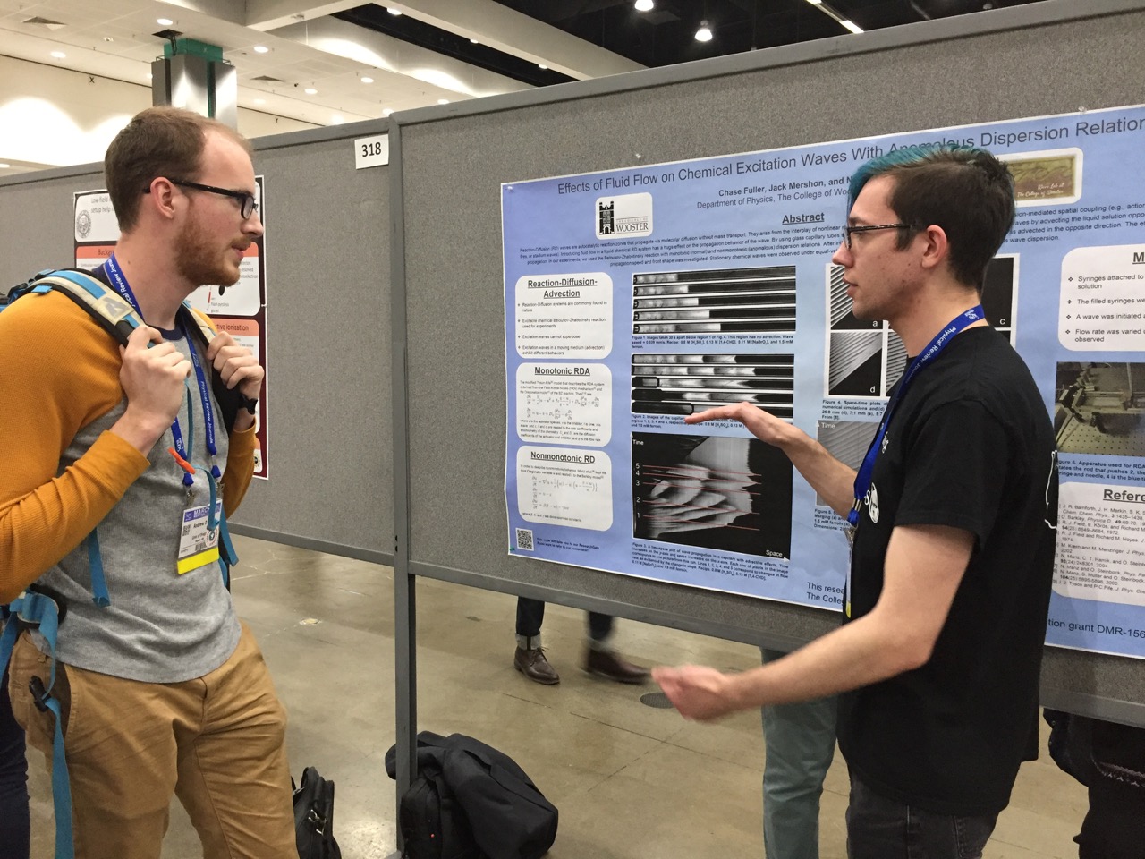
Andrew Blaikie ’13 quizzes Chase Fuller ’19 about BZ waves.
Everybody loves the toys.
Our remaining four students presented their posters and did very well, and had fun gathering up free toys from the vendors in the exhibit hall.
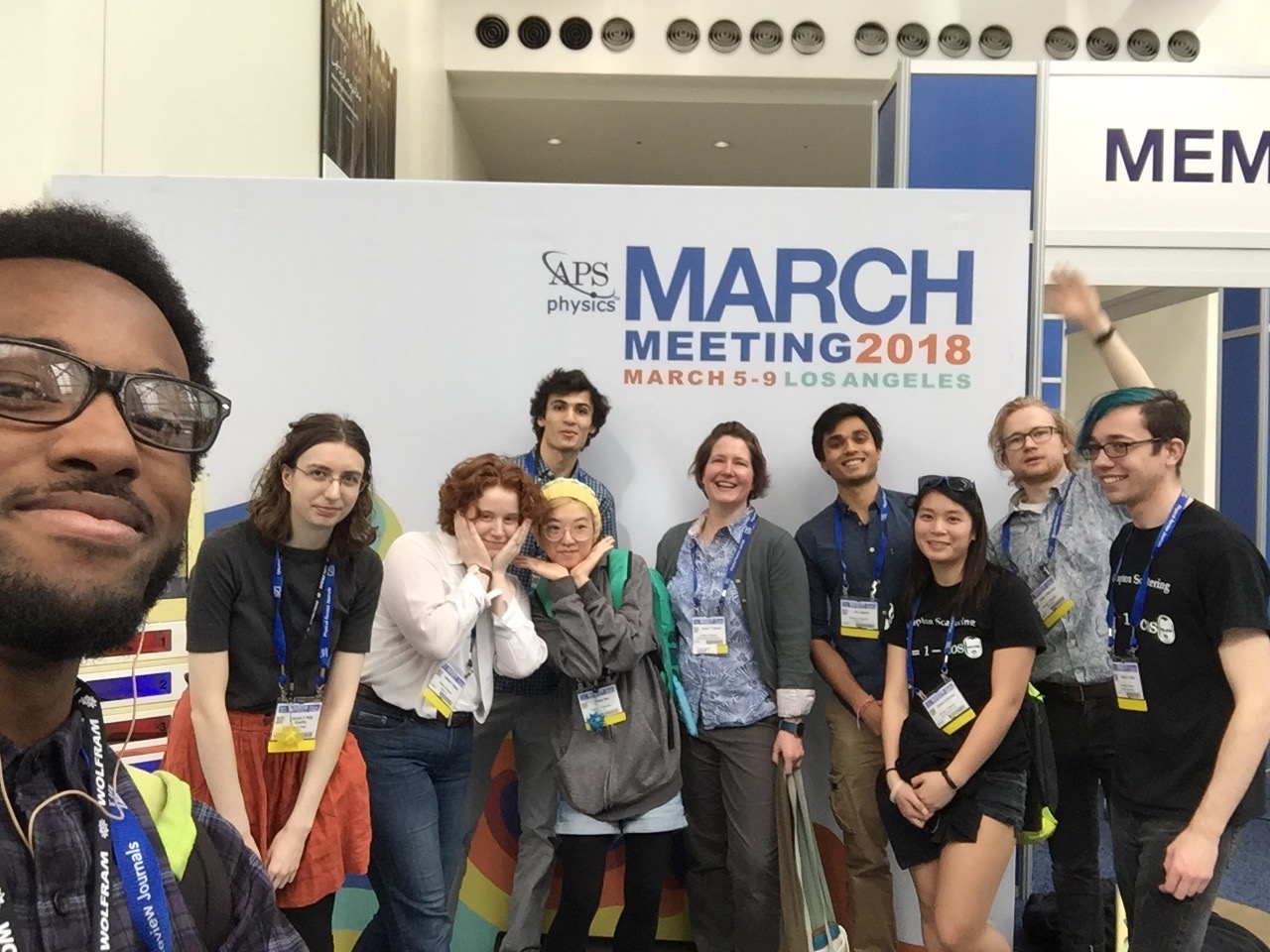
Group selfie, take 2.
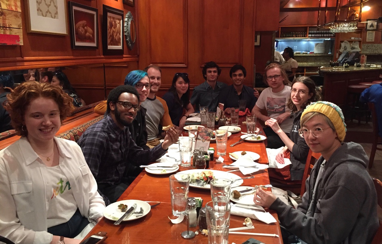
Time for a group photo, and a couple more sessions before a big group dinner. This is always a highlight of the trip (as long as the scheduling works) and this time we got to include alumnus Andrew Blaikie ’13 who is finishing grad school at the University of Oregon.
Wooster physics out for dinner, with bonus alumnus Andrew Blaikie ’13!
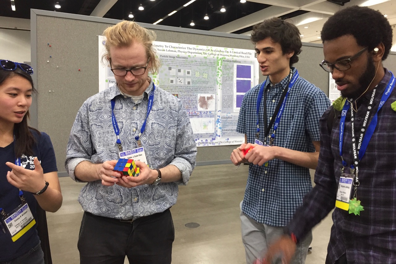
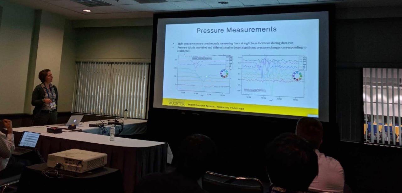
Whew! So much more that I could say, but frankly I’m exhausted. On Thursday, Avi Vajpeyi ’18 presented his bead pile simulation, and I presented the latest experimental bead pile results later in the same session.
Me, taking credit for Gabe’s excellent work
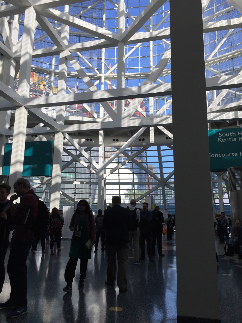
As I said at the start, the March Meeting is exhilarating, but the counterpoint is that it is exhausting. We are starting to hit brain overload here, but fortunately things are winding down. The weather has been lovely, so here’s a final image from the atrium at the convention center. I notice reflections all around, and I liked the blue sky with the reflections in the floor.
Sunlight and reflection in the atrium
Next year in Boston!
Recent Comments
Thanks, Mark! I enjoy reading your posts as well.
Nice post, John! Thanks for writing these. I always enjoy them.


Thanks, Mark! I enjoy reading your posts as well.