Although almost all ordinary mass effectively arises from the kinetic and binding energy of quarks and gluons bound to protons and neutrons in atomic nuclei, the Higgs mechanism does endow some particles like quarks and weakons with intrinsic masses. Here I gently introduce the Higgs mechanism without using loose analogies like vacuum field viscosity.
Stationary Action
For simple systems, the Lagrangian is the difference between the kinetic and potential energies,
L = T – V.
Demand that the action
S = \int dt \,L
be stationary and integrate by parts
0 = \delta S = \int dt \left(\frac{\partial L}{\partial x} \delta x + \frac{\partial L}{\partial \dot x} \delta \dot x \right) = \int dt \left(\frac{\partial L}{\partial x}- \frac{d}{d t}\frac{\partial L}{\partial \dot x} \right)\delta x,
for all variations \delta x, to find the Euler-Lagrange motion equation
\frac{\partial L}{\partial x} = \frac{d}{d t}\frac{\partial L}{\partial \dot x}.
Classic Oscillator
For the simple harmonic oscillator, the Lagrangian
L[x,\dot x] = \frac{1}{2} m \dot x^2 – \frac{1}{2} k x^2
implies the Euler-Lagrange equation
-kx = m \ddot x,
which recovers familiar laws of Hooke and Newton.
Spinless Particle
In 1+1 dimensional spacetime, represent a spinless particle by the quantum of the field \phi[t,x]. In units where c = 1 and \hbar = 1, the Lagrangian
L = \int dx\, \mathcal L = \int dx \left( \mathcal{T} – \mathcal{V} \right)
and the Lagrangian density
\mathcal{L}[\phi, \partial_t \phi, \partial_x \phi] = \frac{1}{2} \left(\partial_t \phi \right)^2 -\frac{1}{2} \left( \partial_x \phi \right)^2 -\frac{1}{2} m^2 \phi^2,
where the signs of the kinetic energy terms reflect the signs of the spacetime interval d\tau^2 = dt^2 – dx^2. The corresponding Euler-Lagrange equation
\frac{\partial \mathcal{L}}{\partial \phi} = \frac{\partial}{\partial t}\frac{\partial \mathcal{L}}{\partial (\partial_t\phi)} + \frac{\partial}{\partial x}\frac{\partial \mathcal{L}}{\partial (\partial_x\phi)}
reduces to the Klein-Gordon equation
-m^2 \phi = \partial_t^2 \phi – \partial_x^2 \phi
or
\left(\partial_t^2 – \partial_x^2 + m^2 \right) \phi = 0.
Assuming wave-particle duality, seek plane wave solutions
\phi = e^{i(-Et+ px)} = e^{i(-Et+ px)/\hbar}= e^{i(-\omega t+ kx)}
to find
\left( (-iE)^2 – (i p)^2 + m^2 \right) \phi = 0
or
E^2 = p^2 + m^2,
where m is the particle mass (and E = m = m c^2 for p = 0).
Nonzero mass determines the simple harmonic oscillator potential energy \mathcal V = m^2 \phi^2 / 2 > 0 and the curvature of the corresponding upright parabola. Zero mass collapses the Klein-Gordon equation to the electromagnetic wave equation.
Symmetry Breaking
Consider the massless Lagrangian density
\mathcal{L}=\mathcal{T} – \mathcal{V} =\frac{1}{2} \left(\partial_t \phi \right)^\dagger \left(\partial_t \phi \right) -\frac{1}{2} \left( \partial_x \phi \right)^\dagger \left( \partial_x \phi \right) + \frac{a}{2} \phi^\dagger \phi – \frac{b}{4} \left( \phi^\dagger \phi \right)^2,
where \phi = \phi_m e^{\phi_a} = \phi_r + i \phi_i , the adjoint \phi^\dagger = \phi^* reduces to complex conjugation, and the parameters a,b > 0. For all complex arguments \phi_a, the potential energy density
\mathcal{V} = – \frac{a}{2} \phi_m^2 + \frac{b}{4} \phi_m^4
depends only on the complex magnitude \phi_m. The vanishing derivative
0 = \frac{d \mathcal{V}}{d \phi_m} = – a \phi_m + b \phi_m^3= \phi_m(- a + b \phi_m^2)
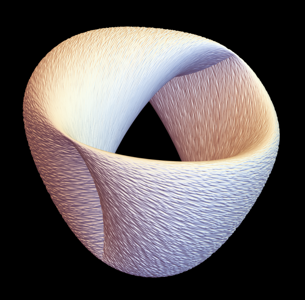
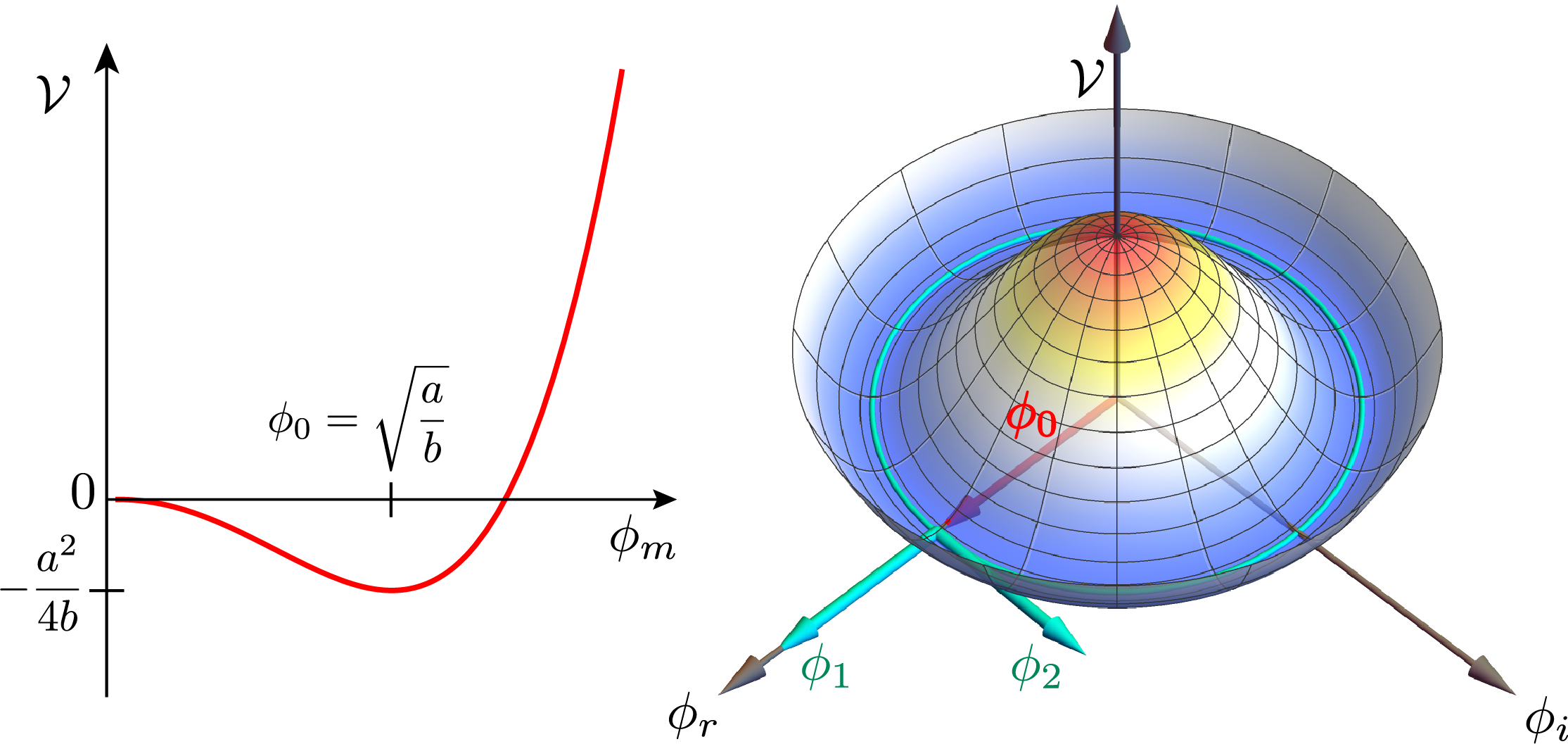
implies local maximum and minimum at \phi_m = 0 and \phi_m = \sqrt{a/b} = \phi_0, as in the figure, where the circular symmetry reflects the invariance of the Lagrangian under global phase (or gauge) transformations \phi \rightarrow \phi \, e^{i \Lambda} = \phi_m e^{i( \phi_a + \Lambda )}.

Higgs potential with minimum at nonzero field (left) and circle of vacua (right).
If the potential is a sombrero, the circular brim are ground or vacua states of nonzero field
\phi_r^2 + \phi_i^2 = \phi_0^2.
Break the circular symmetry by fixing \phi_r = \phi_0 and \phi_i = 0, but allow the field to oscillate radially and shift circularly
\phi[t, x] = \phi_0 + \phi_1[t, x] + i \phi_2[t, x] .
The Lagrangian density becomes
\begin{array}{c}\displaystyle\mathcal{L}= \frac{1}{2} \left(\partial_t \phi_1 \right)^2 -\frac{1}{2} \left( \partial_x \phi_1 \right)^2 – a \phi_1^2 \\ \displaystyle+ \frac{1}{2} \left(\partial_t \phi_2 \right)^2 -\frac{1}{2} \left( \partial_x \phi_2 \right)^2 \\ \displaystyle- \sqrt{a b}\,\phi_1 \left(\phi_1 ^2+\phi_2 ^2\right) -\frac{b}{4} \left(\phi_1 ^2+\phi_2^2\right)^2\\ \displaystyle+ \frac{a^2}{4 b}\end{array}
or
\begin{array}{c}\displaystyle\mathcal{L}= \frac{1}{2} \left(\partial_t \phi_1 \right)^2 -\frac{1}{2} \left( \partial_x \phi_1 \right)^2 – m_1^2 \phi_1^2 \\ \displaystyle+ \frac{1}{2} \left(\partial_t \phi_2 \right)^2 -\frac{1}{2} \left( \partial_x \phi_2 \right)^2 – m_2^2 \phi_2^2 \\ \displaystyle+\text{interaction} + \text{constant},\end{array}
where m_1 = \sqrt{a} > 0 and m_2 = 0.
Summary
Starting with a massless field \phi with nonzero vacuum states, symmetry breaking creates a field \phi_1, corresponding to parabolic radial motion and a massive quantum m_1 > 0, and a field \phi_2, corresponding to constant circular motion and a massless quantum m_2 = 0 (a Goldstone boson). This is the Higgs mechanism of mass endowment.


Thanks, Mark! I enjoy reading your posts as well.