Does a charge in gravity radiate?

Caltech, Saturday night, grad student pizza. The conversation turns to a famous general relativity puzzle: does an electric charge at rest in a gravitational field radiate? According to Einstein’s equivalence principle, a static homogeneous gravitational field is indistinguishable from constant acceleration in empty space, and as is well known, accelerating charges radiate. Does that mean electrons in the table radiate as we eat? Sam says Kip says the electromagnetic field lines bend. We don’t resolve the paradox, and after dinner we return to our grad school homework.

Here, I outline a partial solution to the problem based on the work of Fritz Rohrlich. It’s a long calculation, which I checked using Mathematica. Round parentheses (\ ) group terms, square brackets [\ ] enclose function arguments, and boxes \square enclose matrix elements.

Outline

• Model static homogeneous gravity G with Rohrlich spacetime metric.
• Transform to free-fall coordinates F where G is in hyperbolic motion
• Find hyperbolic geodesics of constant proper acceleration g, as in Fig. 1..
• Find electromagnetic field of charge q at rest in G as observed by F.
• Transform to find electromagnetic field as observed by G.

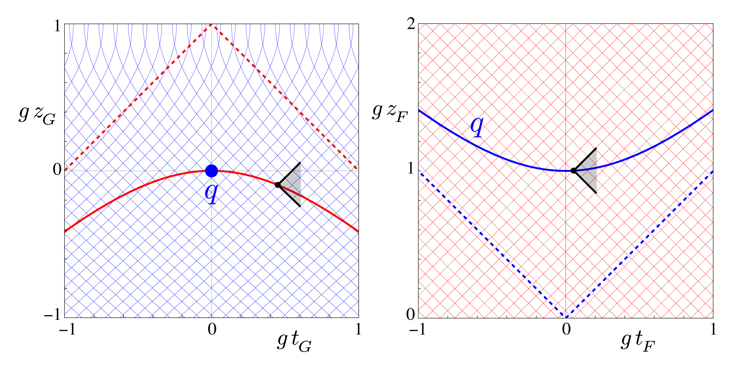
Figure 1: Charge q (blue) at rest in static homogeneous gravitational field (left) and in hyperbolic motion in a freely falling reference frame (right). Gridlines are null (light) lines, which suggest a coordinate singularity at z_G = 1/g, and dashed lines are hyperbola asymptotes. Black lines outline future light cones.

Model Gravity

If g is the non-relativistic gravitational field magnitude, relativistic units implies constant light speed c = 1 with time scale T = c/g_E \approx 1~\text{year}, and length scale L = c^2/g_E \approx 1~\text{light-year}. Restricting spatial motion to the vertical z direction implies cylindrical symmetry, so use cylindrical spacetime coordinates

x^\mu = \boxed{\begin{array}{c} x^0 \\ x^1 \\ x^2 \\ x^3 \\\end{array}} = \boxed{\begin{array}{c} ct \\ \rho \\ \phi \\ z \\\end{array}} = \boxed{\begin{array}{c} t \\ \rho \\ \phi \\ z \\\end{array}} = \boxed{\begin{array}{c} t \\ \vec x \\ \end{array}}.

The line element

\text d\tau^2 = \sum_{\mu=0}^3 \sum_{\nu=0}^3 g_{\mu\nu} \text dx^\mu \text dx^\nu = g_{\mu\nu} \text dx^\mu \text dx^\nu

gives the proper time d\tau between nearby events. Model a free-fall spacetime using the Minkowski metric tensor with matrix representation

g^F_{\mu\nu} = \boxed{\begin{array}{cccc} 1 & 0 & 0 & 0 \\ 0 & -1 & 0 & 0\\0 & 0 & -\rho^2 & 0 \\0 & 0 & 0 & -1 \\ \end{array}} = \eta_{\mu\nu},

and line element

\text d\tau^2 = \text dt^2-\text d\rho^2-\rho^2\text d\phi^2-\text dz^2 = \text dt^2-\text d\vec x^2,

where

\frac{1}{\gamma^2} = \left( \frac{\text d\tau}{\text dt} \right)^2 = 1-\left( \frac{\text d\vec x}{\text dt} \right)^2.

Simply model gravity using the Rohrlich metric tensor with matrix representation

g^G_{\mu\nu} = \boxed{\begin{array}{cccc} u[z_G]^2 & 0 & 0 & 0 \\ 0 & -1 & 0 & 0 \\0 & 0 & -\rho^2 & 0 \\0 & 0 & 0 & -u'[z_G]^2/g^2 \\ \end{array}} = \boxed{g^{\mu\nu}_G}^{-1},

where

u[z] = \text{sech}\left[\sqrt{(1-g z)^2-1}\right] = 1 + g z + O[z^2].

The Rohrlich spacetime is static (independent of time t), homogeneous (independent of horizontal coordinates x = \rho\cos\phi, y=\rho\sin\phi), and depends only on height z and parameter g.

Free fall

Newtonian free fall \vec x[t] satisfies \text d^2\vec x / \text dt^2 = \vec 0. More generally, geodesic motion x^\alpha[\tau] satisfies

\frac{\text d^2 x^\alpha}{\text d \tau^2} = -\Gamma^\alpha_{\mu\nu} \frac{\text dx^\mu}{\text d \tau}\frac{\text d x^\nu}{\text d \tau},

with implied sums over the repeated indices, where the connection coefficients

\Gamma^\alpha_{\beta\gamma} = \frac{1}{2}g^{\alpha\delta}\left(\frac{\partial g_{\delta\beta}}{\partial x^\gamma} + \frac{\partial g_{\gamma\delta}}{\partial x^\beta} – \frac{\partial g_{\beta\gamma}}{\partial x^\delta} \right)

encode the rates of basis vector component changes with coordinate changes. Here, the solutions

\boxed{\begin{array}{c} t_G \\ \rho_G \\ \phi_G \\ z_G \end{array}} = \boxed{\begin{array}{c} \text{arctanh}[g\tau]/g \\ 0 \\ 0 \\ (1-\sqrt{1+\text{arctanh}[g\tau]^2})/g \end{array}}

imply hyperbolic motion

(z_G-1/g)^2-t_G^2 = 1/g^2,

where

z_G = \frac{1-\sqrt{1+g^2 t_G^2}}{g} = -\frac{1}{2} g t_G^2 + O[t_G^4],

as designed.

Transform to free fall frame

By the equivalence principle, a freely falling test particle defines a locally flat or inertial system. Equating the free and gravity line elements

\begin{aligned}\text d\tau^2 &= \text dt_F^2-\text d\rho_F^2-\rho_F^2 \text d\phi_F^2-\text dz_F^2 \\ &= u[z_G]^2 \text dt_G^2-\text d\rho_G^2-\rho_G^2 \text d\phi_G^2-\frac{u^\prime[z_G]^2}{g^2} \text dz_G^2,\end{aligned}

implies the transformation

x^\mu_F = \boxed{\begin{array}{c} t_F \\ \rho_F \\ \phi_F \\ z_F \end{array}} = \boxed{\begin{array}{c} \sinh[g t_G] u[z_G]/g \\ \rho_G \\ \phi_G \\ \cosh[g t_G] u[z_G] / g \end{array}}

with Jacobian

\underset{F\leftarrow G}{J^\mu_\nu} = \frac{\partial x^\mu_F}{\partial x^\nu_G} = \boxed{\begin{array}{cccc} \cosh[gt_G]u[z_G] & 0 & 0 & \sinh[gt_G]u^\prime[z_G]/g \\ 0 & 1 & 0 & 0\\0 & 0 & 1 & 0 \\ \sinh[gt_G]u[z_G] & 0 & 0 &\cosh[gt_G]u^\prime[z_G]/g \end{array}}

Thus, the charge q at rest in G at x_G = y_G = z_G = 0 moves in F along the hyperbola

z_F^2\ -\ t_F^2 = u[z_G]^2/ g^2 = u[0]^2/ g^2 = 1 / g^2,

where

z_F = \frac{\sqrt{1+g^2 t_F^2}}{g} = \frac{1}{g}+\frac{1}{2} g t_F^2 + O[t_F^4].

Generally, the spacetime acceleration A^\mu = d^2 x^\mu / d^2\tau^2 implies the Lorentz-invariant

\sqrt{-A^\mu A_\mu} = \sqrt{-g_{\mu\nu}A^\mu A^\nu} = \frac{\ddot{z}}{(1-\dot{z}^2)^{3/2}} = \gamma^3 \ddot z,

for \ddot z >0, where the over-dots indicate differentiation with respect to time t. Here, the proper acceleration of q fixed in G

\ddot z_G = \gamma_G^3 \ddot z_G^{} = \gamma_F^3 \ddot z_F = \frac{\ddot{z}_F}{(1-\dot{z}_F^2)^{3/2}} = g

is constant, as expected. (Furthermore, 1 < \gamma_F implies \ddot z_F < g, and \ddot z_F \rightarrow 0 as \dot z_F \rightarrow c, so F never observes q superluminal.)

Electromagnetic fields in free fall frame

Generally, for a charge q in arbitrary motion x^\mu_q[\tau], the Coulomb potential \varphi = q / r generalizes to the Liénard-Wiechert potential

\mathcal{A}^\mu = q\frac{U^\mu}{R^\nu U_\nu} \bigg|_{t_r} = q\frac{U^\mu}{g_{\alpha\beta}R^\alpha U^\beta} \bigg|_{t_r},

where the spacetime velocity U^\mu = dx^\mu_q / d\tau, the spacetime displacement R^\mu = x^\mu-x^\mu_q, and because electromagnetic “news” travels at light speed, the right side is evaluated at the earlier, retarded time t_r defined implicitly by

t-t_r = \big| \vec x-\vec x_q[t_r] \big| / c.

Let the cylindrical coordinates of the field point at time t be \{\rho, \phi, z\}, and define

\begin{aligned}\delta^2 &= -t^2 + \rho^2 + z^2 + g^{-2}, \\ \Delta^2 &= +t^2 + \rho^2-z^2 + g^{-2}, \\ d^2 &= +t^2-\rho^2-z^2 + g^{-2}, \\ \xi &= \sqrt{4 g^{-2} \rho^2 +d^2}.\end{aligned}

Here, for the charge’s hyperbolic motion in the free-fall frame, explicitly solving for the retarded time is possible, and

t_F-t_r = \sqrt{\rho_F^2 +(z_F-\sqrt{g^{-2}+t_r^2}\,)^2}

implies

t_r = \frac{t_F\delta_F^2-z_F\xi_F}{2(z_F^2-t_F^2)}.

Evaluating the Liénard-Wiechert potential at this time gives

U^\mu_F = \frac{g}{2(z_F^2-t_F^2)}\boxed{\begin{array}{c} z_F \delta_F^2-t_F\xi_F \\ 0 \\ 0 \\ t_F \delta_F^2-z_F \xi_F \end{array}}

and

R^\mu_F = \frac{1}{2(z_F^2-t_F^2)}\boxed{\begin{array}{c} z_F \xi_F-t_F\Delta_F^2 \\ 2\rho_F(z_F^2-t_F^2) \\ 0 \\ t_F \xi_F-z_F \Delta_F^2 \end{array}}

and finally

\mathcal{A}^\mu_F = \frac{q}{\xi_F(z_F^2-t_F^2)}\boxed{\begin{array}{c} z_F \delta_F^2-t_F\xi_F \\ 0 \\ 0 \\ t_F \delta_F^2-z_F \xi_F^2 \end{array}}.

Differentiating the electromagnetic field tensor

\boxed{\begin{array}{cccc}0 & +\mathcal{E}_\rho & +\mathcal{E}_\phi & +\mathcal{E}_z \\-\mathcal{E}_\rho & 0 & -\mathcal{B}_z & +\mathcal{B}_\phi \\-\mathcal{E}_\phi & +\mathcal{B}_z & 0 & -\mathcal{B}_\rho \\-\mathcal{E}_z & -\mathcal{B}_\phi & +\mathcal{B}_\rho & 0 \end{array}}_F = \mathcal{F}_F^{\mu\nu} = \frac{\partial \mathcal{A}_F^\nu}{\partial x_F^\mu}-\frac{\partial \mathcal{A}_F^\mu}{\partial x_F^\nu},

generates the electric and magnetic field vectors

\begin{aligned}\vec\mathcal{E}_F &= \frac{4 g^{-2} q}{\xi_F^3} \boxed{\begin{array}{c}2\rho_F z_F \\0\\-\Delta_F^2 \end{array}}, \\ \vec\mathcal{B}_F &= \frac{4 g^{-2} q}{\xi_F^3} \boxed{\begin{array}{c}0 \\2\rho_F t_F\\0 \end{array}}, \end{aligned}

for z_F> t_F, as in Fig. 2. The directional energy flux density or Poynting vector

\vec\mathcal{S}_F = \vec\mathcal{E}_F \times \vec\mathcal{B}_F = \frac{32 g^{-4} q^2 t_F \rho_F}{\xi_F^6} \boxed{\begin{array}{c}\Delta_F^2 \\0 \\ 2\rho_F z_F \end{array}}.

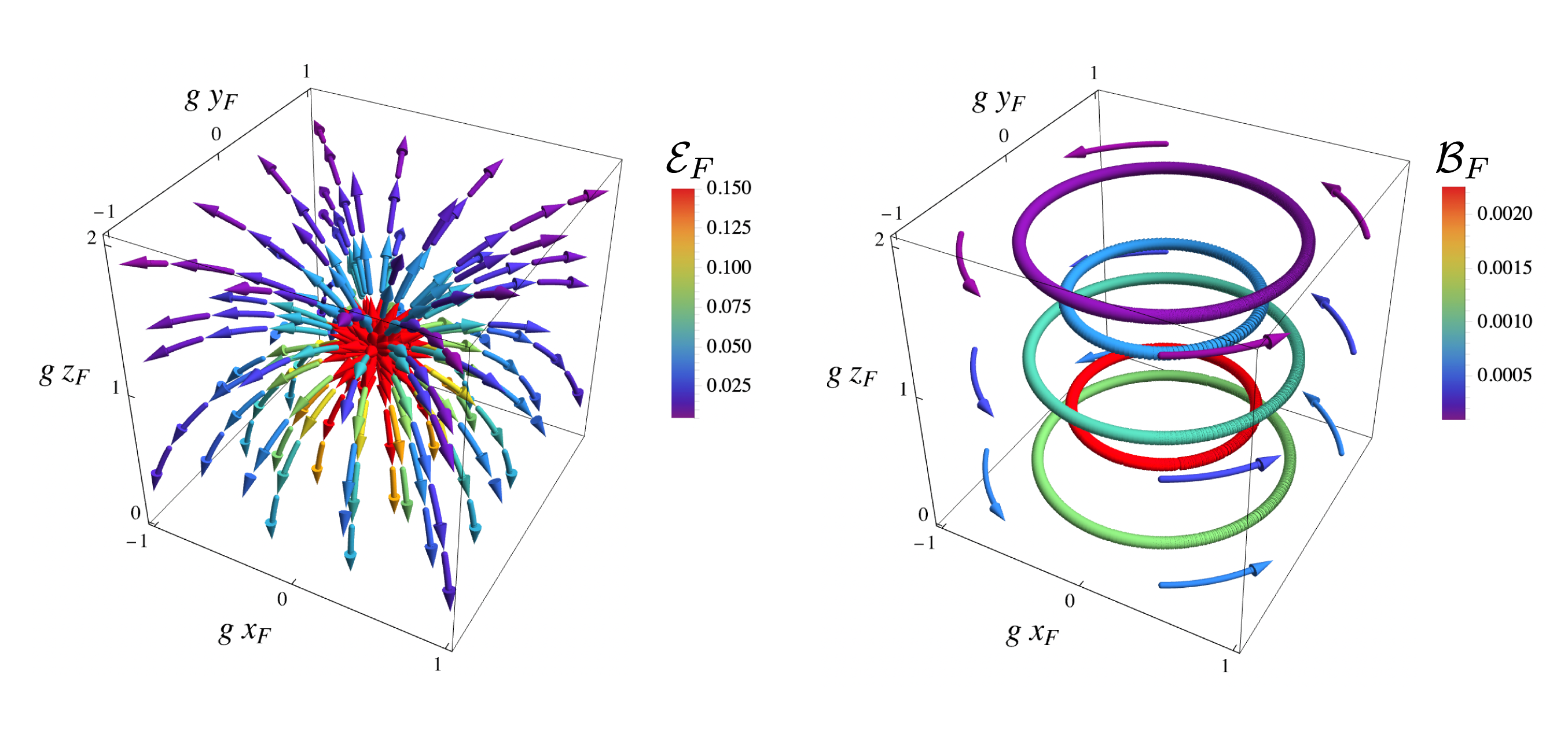
Figure 2: Electric and (nonzero) magnetic fields in the free fall frame F for a charge q at rest in G and accelerating upward in F. Parameters are q=1, g = 0.2, and t_F=0.1.

Electromagnetic fields in gravity frame

The electromagnetic field transformed to the gravity frame is

\boxed{\begin{array}{cccc}0 & +\mathcal{E}_\rho & +\mathcal{E}_\phi & +\mathcal{E}_z \\-\mathcal{E}_\rho & 0 & -\mathcal{B}_z & +\mathcal{B}_\phi \\-\mathcal{E}_\phi & +\mathcal{B}_z & 0 & -\mathcal{B}_\rho \\-\mathcal{E}_z & -\mathcal{B}_\phi & +\mathcal{B}_\rho & 0 \end{array}}_G = \mathcal{F}_G^{\mu\nu} = J^{\mu}_\alpha J^{\nu}_\beta \mathcal{F}_F^{\alpha\beta},

with implied sums over repeated indices. Hence,

\begin{aligned}\vec\mathcal{E}_G &= \frac{4 g^{-2}q}{\xi_G^3} \frac{\text{sech}\chi_G}{\chi_G} \boxed{\begin{array}{c}2\rho_G (z_G \cosh[g t_G]-t_G\sinh[g t_G])\chi_G \\ 0 \\ -\Delta_G^2 (1-g z_G)\text{sech}\chi_G \tanh\chi_G \end{array}}, \\ \vec\mathcal{B}_G &= \boxed{\begin{array}{c}0 \\ 0 \\ 0 \end{array}}, \end{aligned}

where \chi = \sqrt{(1-g z)^2-1}, as in Fig. 3. As a check,

\lim_{g\rightarrow 0} \vec\mathcal{E}_G = \frac{q}{(z_G^2 + \rho_G^2)^{3/2}} \boxed{\begin{array}{c}\rho_G \\ 0 \\ z_G \end{array}} = \frac{q}{z_G^2 + \rho_G^2} \frac{\rho_G \hat\rho + z_G \hat z}{\sqrt{z_G^2 + \rho_G^2}} = \frac{q}{r_G^2} \hat r_G,

as expected. The Poynting vector

\vec\mathcal{S}_G = \vec\mathcal{E}_G \times \vec\mathcal{B}_G = \boxed{\begin{array}{c} 0 \\ 0 \\ 0 \end{array}}.

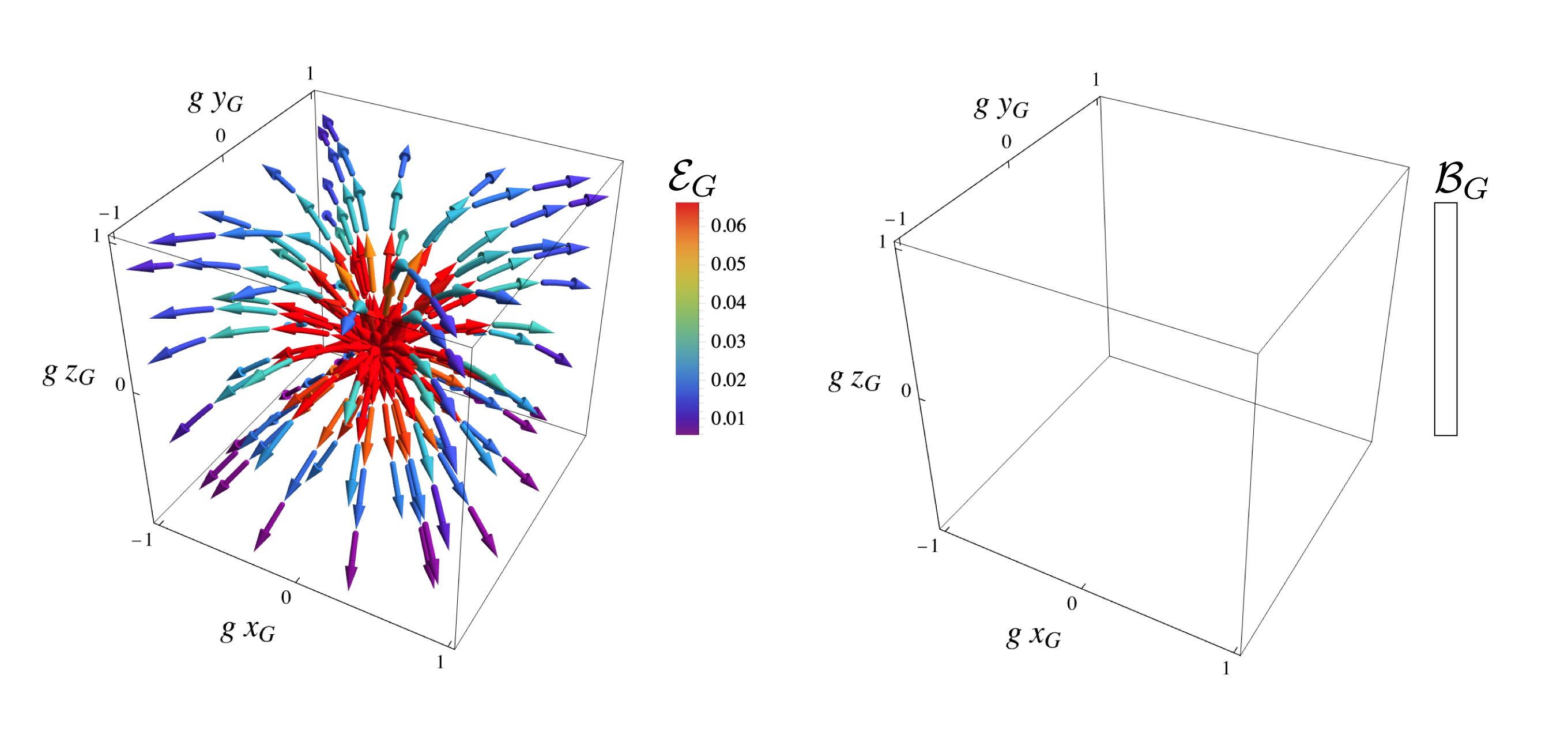
Figure 3: Electric and (zero) magnetic fields in the gravity frame G for a charge q=1 at rest in G with g = 0.2.

Summary

Kip was right; the field lines bend (downward). But also, radiation is not a frame-invariant concept.