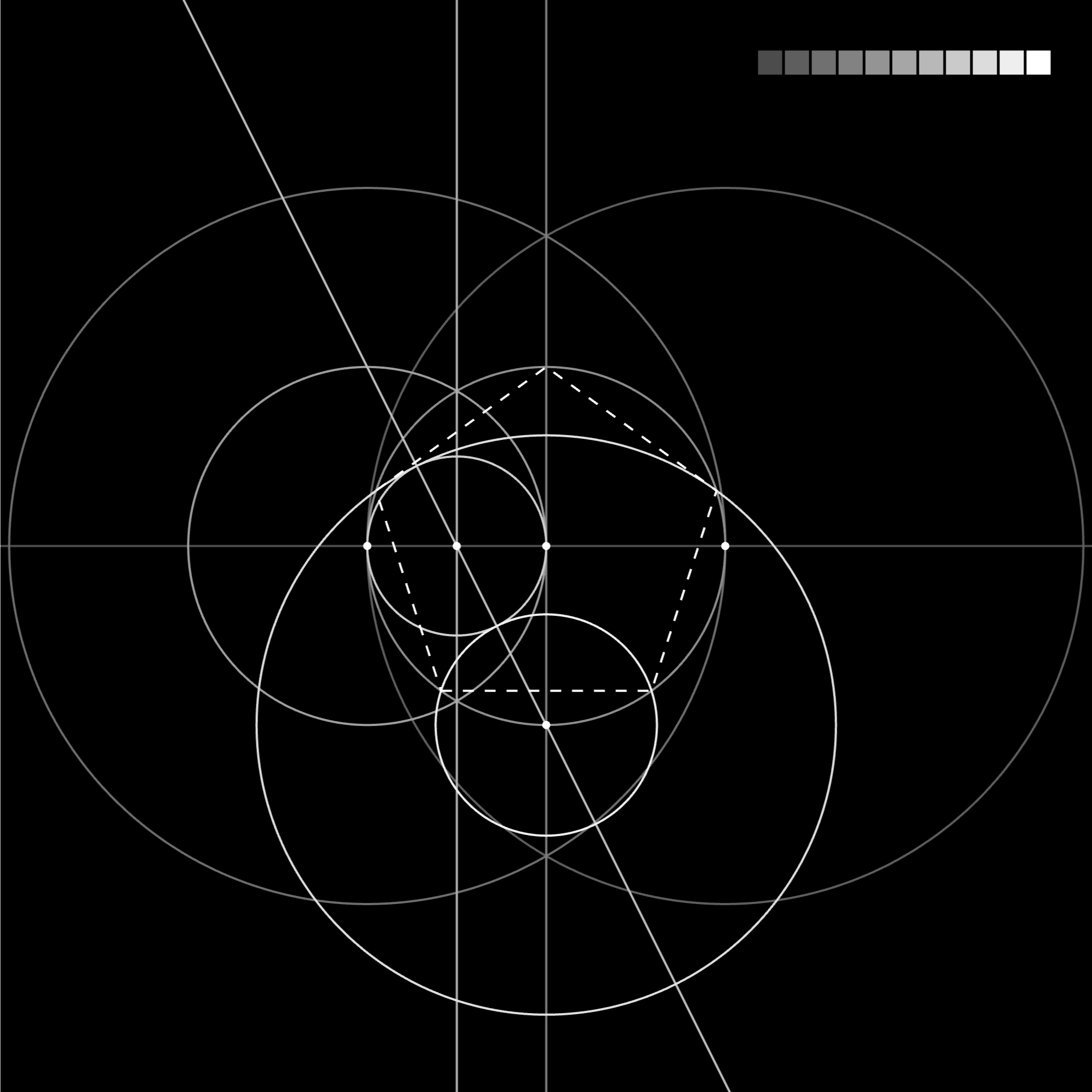
A highlight of Euclid’s Elements is the exact construction of a regular pentagon using a straight edge and a compass. But I’ve noticed recently that some of the pentagon constructions on YouTube are merely approximations – and are not advertised or understood as such. Furthermore, many of these constructions require non-collapsible compasses, which can “carry” lengths from one place to another, thereby shortcutting the classical process.
Here I present a rigorous construction of a pentagon by just drawing lines and circles through intersections of previous lines and circles (from a pre-existing pair of points), which can be replicated by a straight edge and the ancient Greekcollapsible compass. Rather than animate the construction, I color code the lines and circles by hues or grays in order of execution. I implement the construction in the Wolfram Language, formerly known as Mathematica, and thereby confirm the exactness of the result.
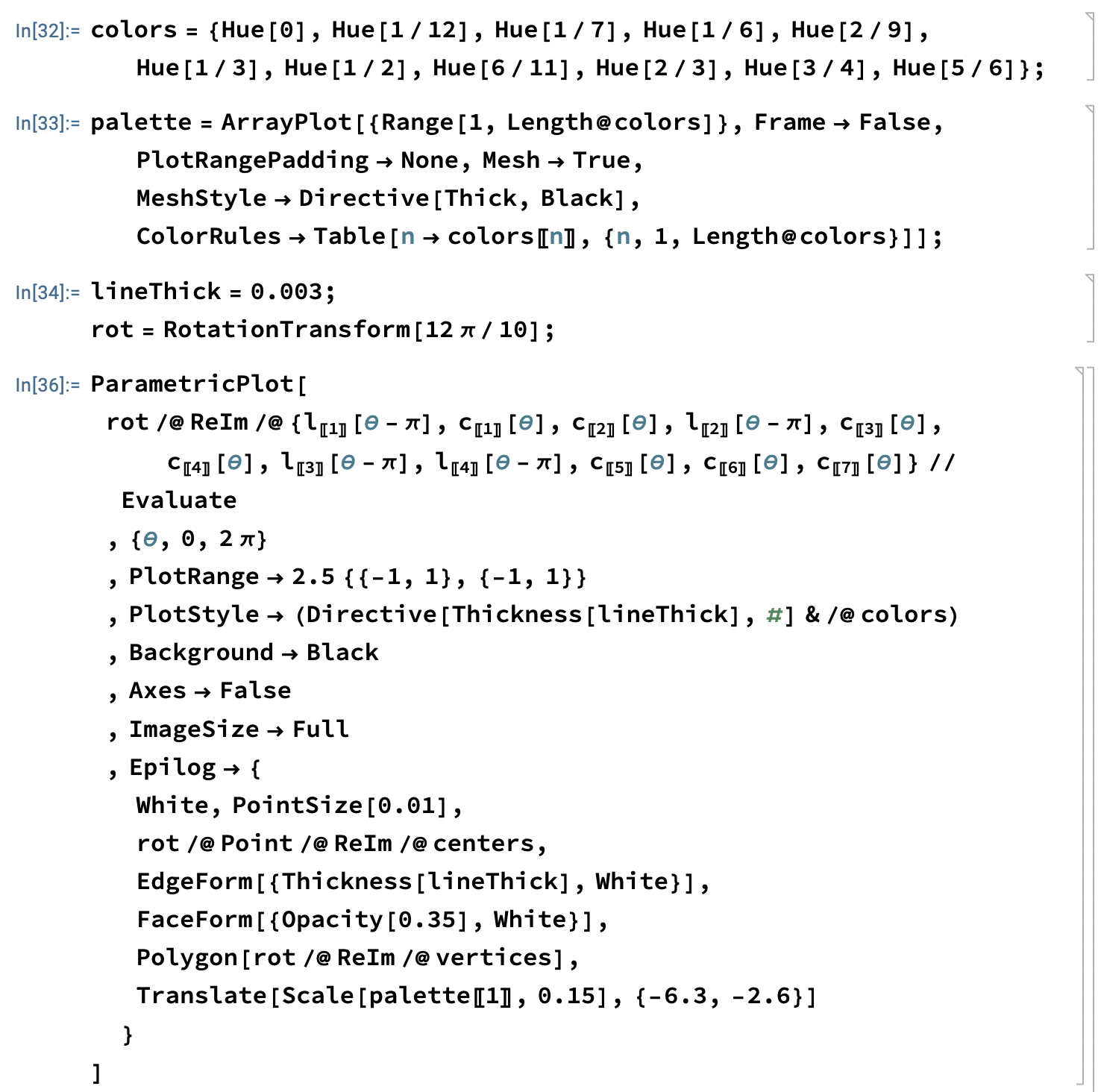
For variety, the hues version is rotated with respect to the grays version, and the code follows the figures.
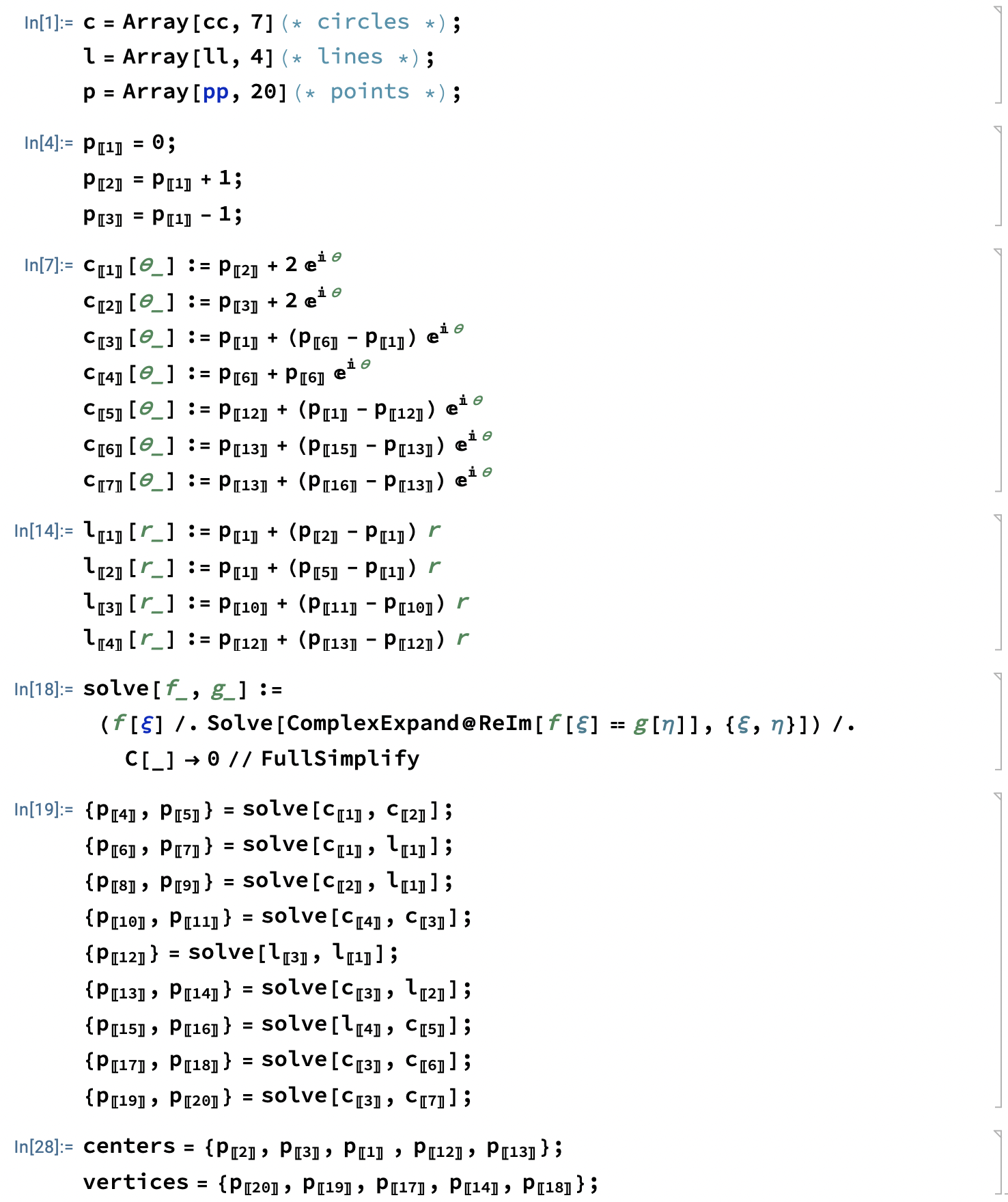
In Mathematica, I define circles, lines, and points as complex numbers and solve for intersections algebraically.
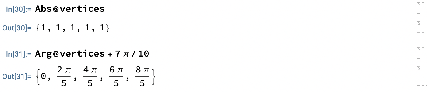
The moduli and arguments of the complex vertices verify the pentagonal geometry.
The ParametricPlot function draws the 7 circles and 4 lines, with white dots at circle centers.
I recently coauthored an article in the InternationalJournal of Bifurcation and Chaos that reports efficiently performing logic with a simple nonlinear electronic device that exhibits negative resistance, something I had previously theorized.
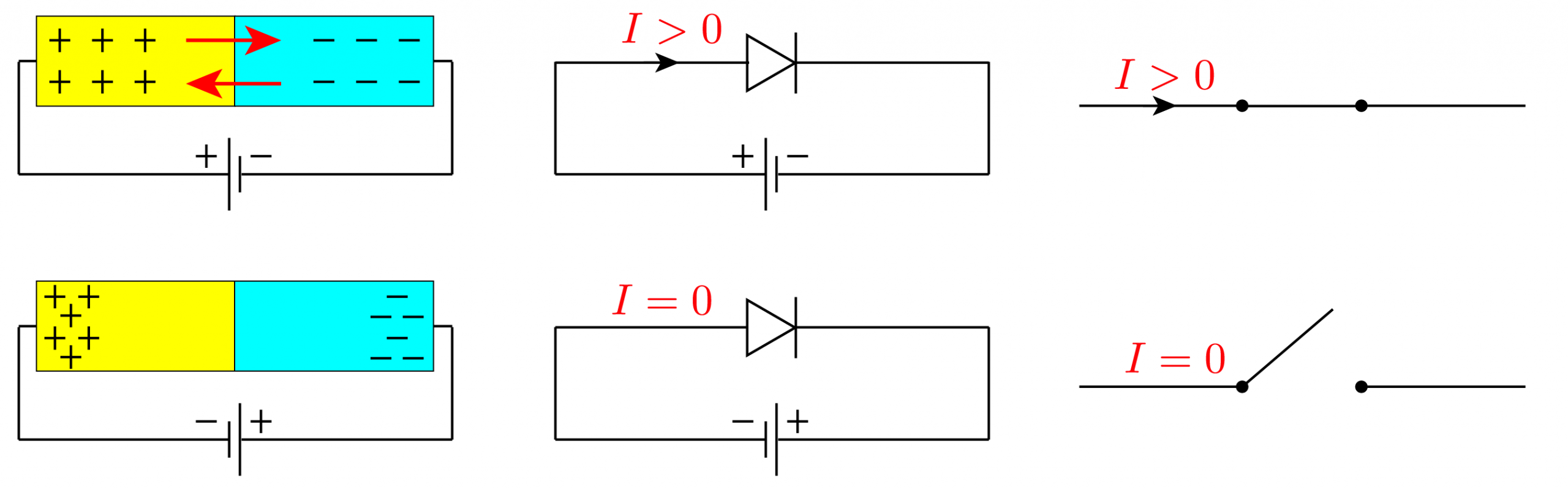
At the heart of the device is a single p-n junction, which is formed by a silicon semiconductor crystal doped with impurity atoms (like boron or antimony) so the n-type side contributes negative charges called electrons to conduction, while the p-type side contributes missing electrons called holes, which act like positive charges. Depending on the polarity of the attached battery, the intermediate depletion layer contracts or expands, and the junction acts like a switch or valve called a diode, either conducting current or blocking it.
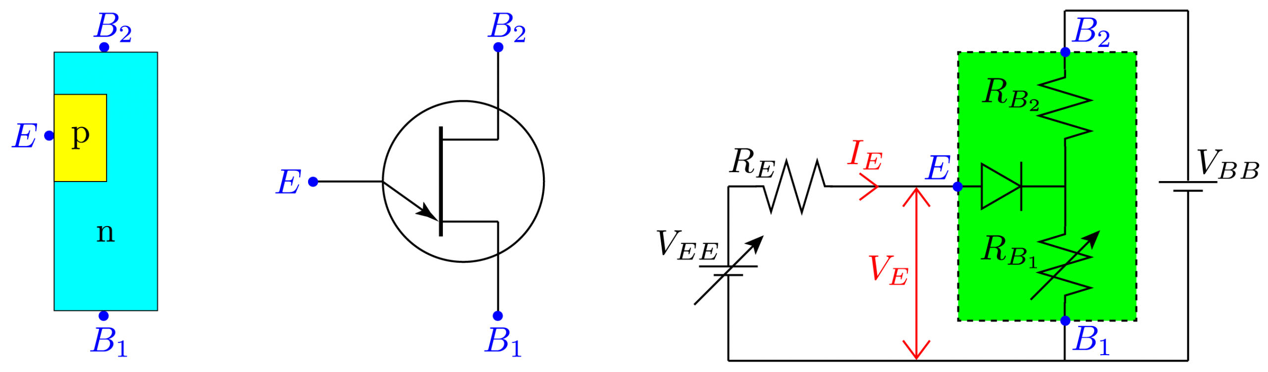
The Uni-Junction Transistor (UJT) is a singleasymmetric p-n junction, whose equivalent circuit features an ideal diode that outputs to two internal resistors, the bottom of which is variable. The three attachment points are conventionally called the side “emitter” E, the bottom “base” B_1, and the top “base” B_2.
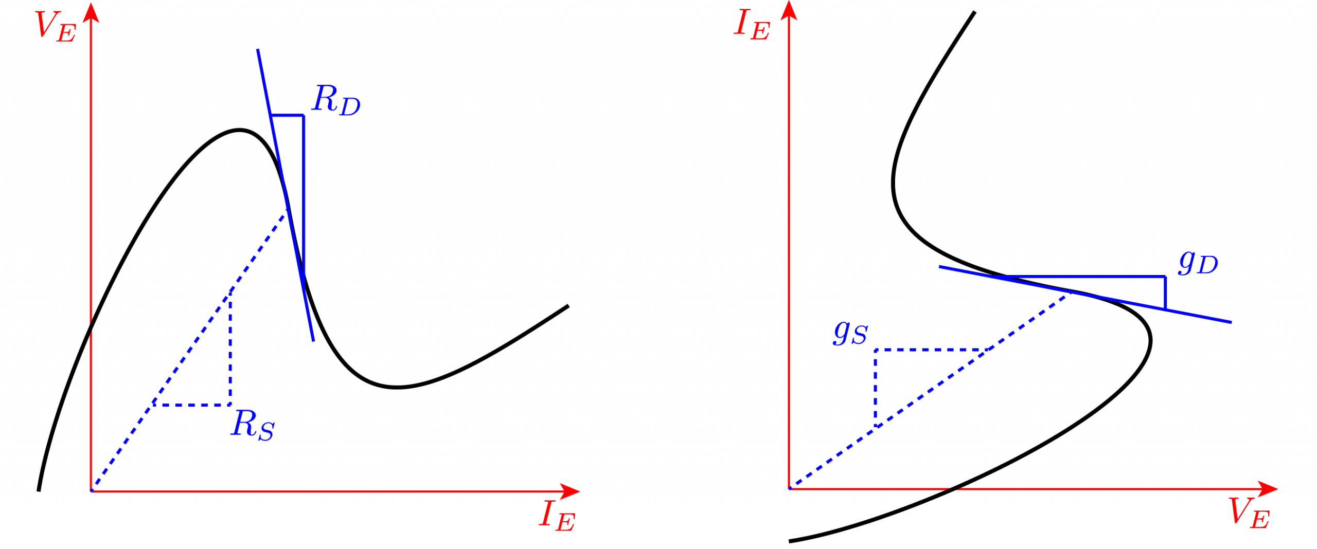
Power the UJT by a static voltage V_{BB} between the bases so B_2 > B_1, and control the emitter voltage V_E and current I_E with the variable voltage V_{EE} via a resistor R_{E}. Varying V_{EE} reveals the BJT characteristic voltage-current VI curve (and IV curve) labeled with static resistanceR_S = V/I and differential or dynamic resistance R_D = dV/dI (and the corresponding conductances g = 1/R). The current I_E versus voltage V_E is multivalued.
For small V_{EE} the p-n junction is reversed biased, and a small current I_E leaks backward through it. For larger V_{EE}, the p-n junction becomes forward biased, triggering it to inject holes into the n-type bar, where the extra charge carriers dramatically increase conductivity, decreasing the voltage V_{E} while increasing the current I_{E}, in a region of negative differential resistance.
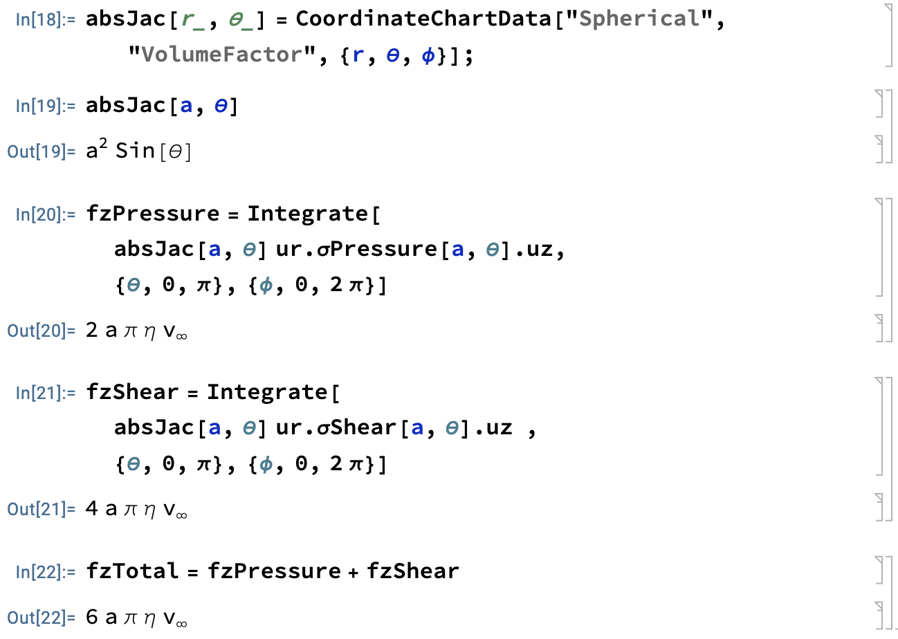
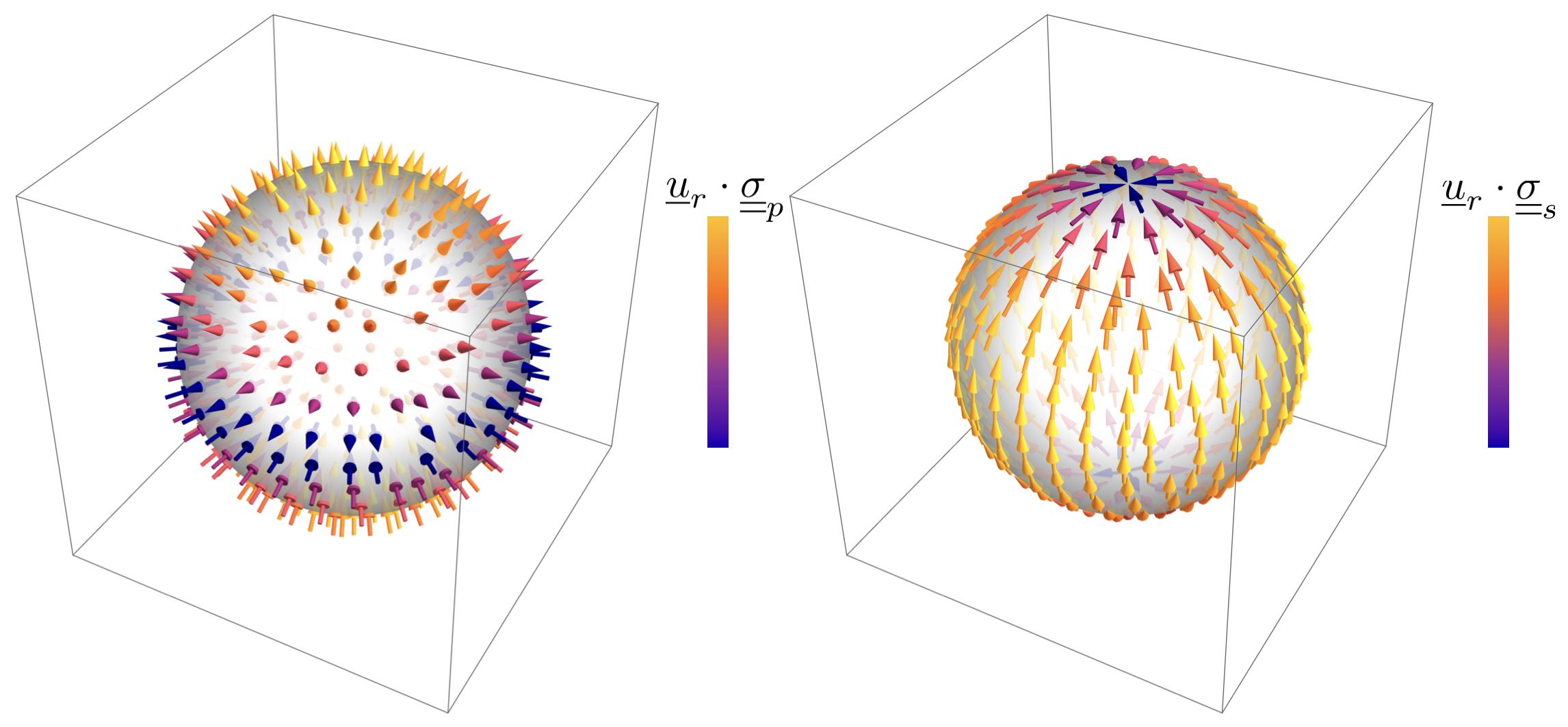
Introductory physics often assumes without proof that the drag force on an object is proportional to its velocity, at least for smooth or laminar flow. In particular, a sphere of radius a falling slowly with velocity \underline v in air of viscosity\eta experiences a drag force
\underline{F} = -6\pi \eta a \underline{v},
which was first derived by GeorgeStokes in 1851. Here is a digestible derivation of the force on an idealized sphere in an upward flowing fluid using Mathematica, including motivation for the underlying Navier-Stokes fluid-flow equations.
Vectors (with singly-indexed components that can be arranged in column matrices) are underlined while second-rank tensors (with doubly-indexed components that can be arranged in square matrices) are doubly-underlined.
Navier-Stokes Equations
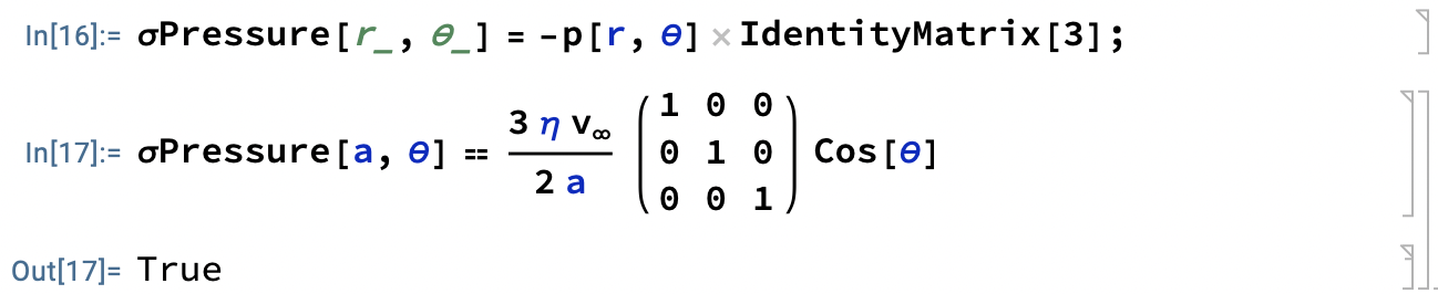
Stress tensor
Recall that pressure perpendicular to the x-direction due to force in the x-direction is
p_x = \frac{dF_x}{da_x},
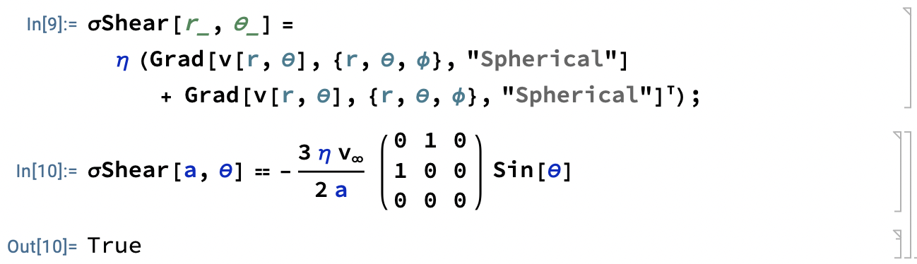
and the shear perpendicular to the y-direction due to velocity changes in the x-direction is
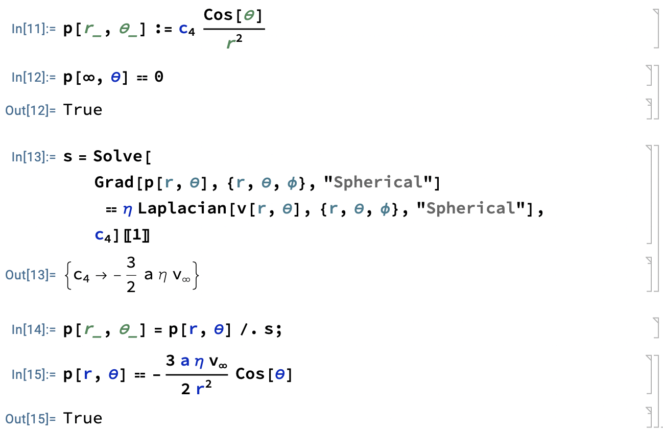
plus boundary conditions determine the fluid pressure p and velocity \underline{v}.
Pressure and Velocity
Although the computation can be done by hand (as Stokes did), Mathematica eases the workload.
Coordinates
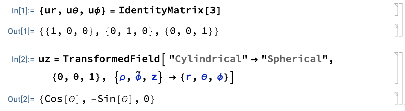
Due to the sphere, introduce spherical coordinates \{r, \theta,\phi \} with unit vectors \{\underline{u}_r, \underline{u}_\theta, \underline{u}_\phi \}, and due to the distant uniform flow, introduce the cylindrical unit vector \underline{u}_z.
Solve Eq. (1) for Velocity
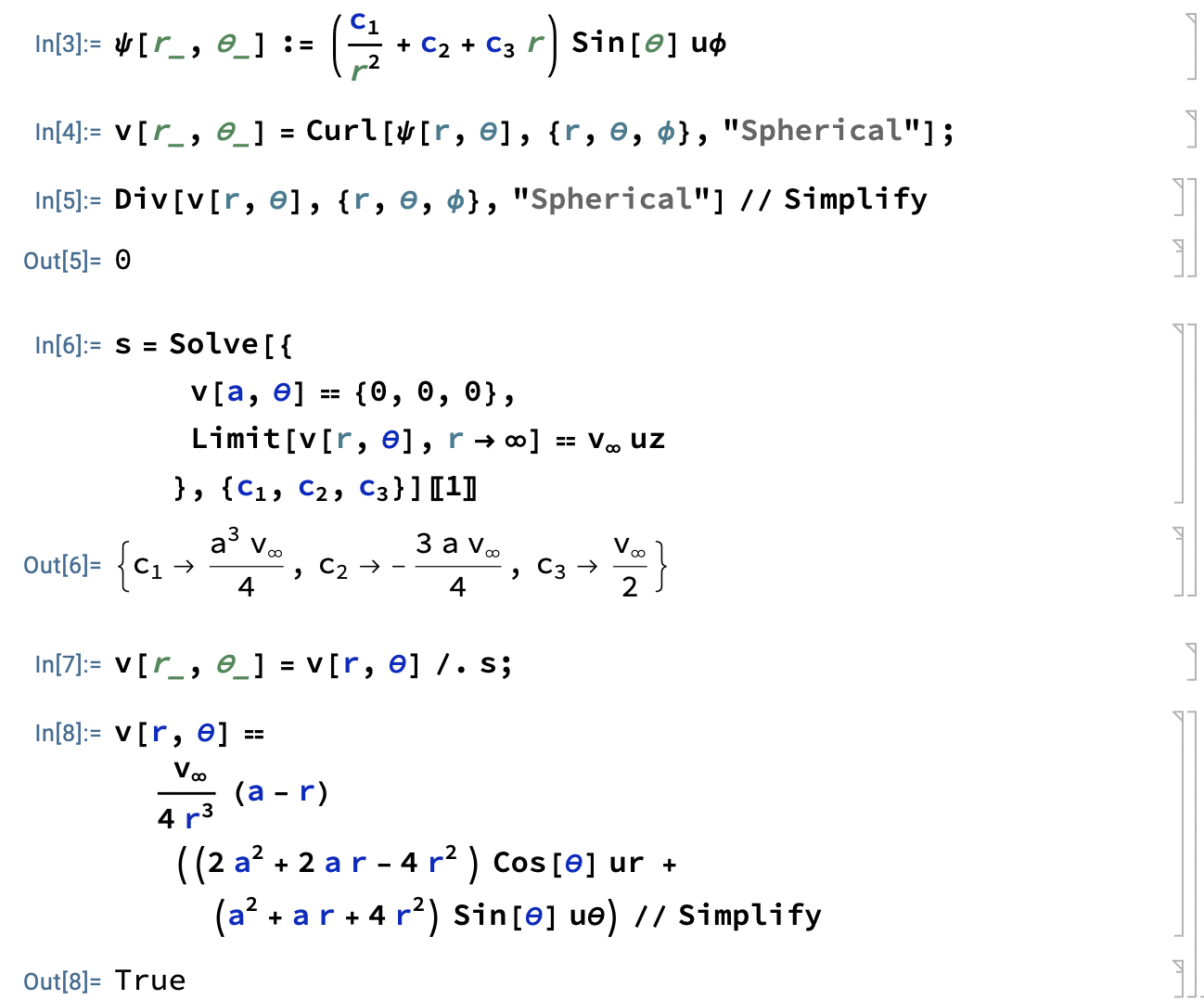
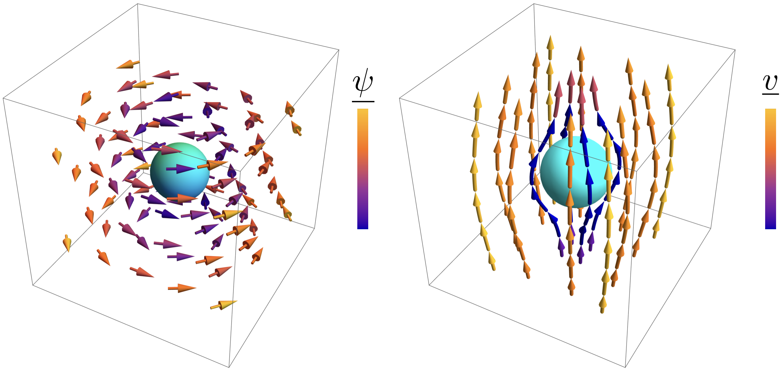
Because the divergence of any curl vanishes, take the fluid velocity (with respect to the sphere) to be the curl of a vector field \underline{v} = \underline{\nabla} \times \underline{\psi}, where the educated guess
\underline{\psi}(r,\theta) = \underline{u}_\theta \left( \frac{c_1}{r^2}+c_2 + c_3 r \right) \sin\theta,
subject to the sticky boundary at the sphere and the uniform boundary at infinity, implies
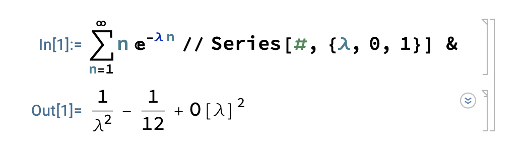
Why is minus-one-twelfth associated with the sum of the natural numbers? It’s the constant term in the series expansion of the corresponding smoothed or regularized sum! Introduce a decay factor, and in the limit of vanishing decay, the finite-non-zero part of the resulting sum is minus-one-twelfth, as one can quickly verify in Mathematica using (for example) an exponential decay:
In more detail, let the sum of natural numbers
S = \sum_{n=0}^\infty n = 1+2+3+\cdots = \infty.
To elucidate this divergent sum and identify the little bit of finiteness that can be extracted from it, introduce an exponential convergence factor and integrate to find
where R denotes regularized, renormalized, and remainder. R also denotes Ramanujan, who discovered this association without any formal mathematical training.
Known for thousands of years, hundreds of proofs of the Pythagorean theorem have been published, including one by U.S. President James Garfield. Here I animate three of my favorites. Each shows that the sum of the squares of the lengths of the legs of a right triangle equals the square of the length of its hypotenuse,
a^2+b^2=c^2.
Without loss of generally, assume a \le b < c. You may need to click or tap the figures to trigger the animations.
Shuffle
Quadruplicate the triangle, and arrange the copies along the edges of a square so they bound a rotated square of area c^2 (colored cyan in the animation below). Shuffle the triangles to form two rectangles that bound two smaller squares of size a^2 and b^2. Since shuffling does not change the exposed (cyan) area, a^2+b^2=c^2
Rescale
Triplicate the triangle, rescale one copy by the hypotenuse length c, a second by the leg length a, and a third by the leg length b. Flip the leg triangles and join all 3 copies to form a rectangle with opposite sides of length a^2+b^2=c^2.
Unfold
Guided by a perpendicular from the right angle to the hypotenuse, unfold the triangle so the original is surrounded by 3 similar triangles. The sum of the areas of the unfolded leg triangles equals the area of the unfolded hypotenuse triangle, and since the areas are proportional to the those of the corresponding squares, a^2+b^2=c^2.
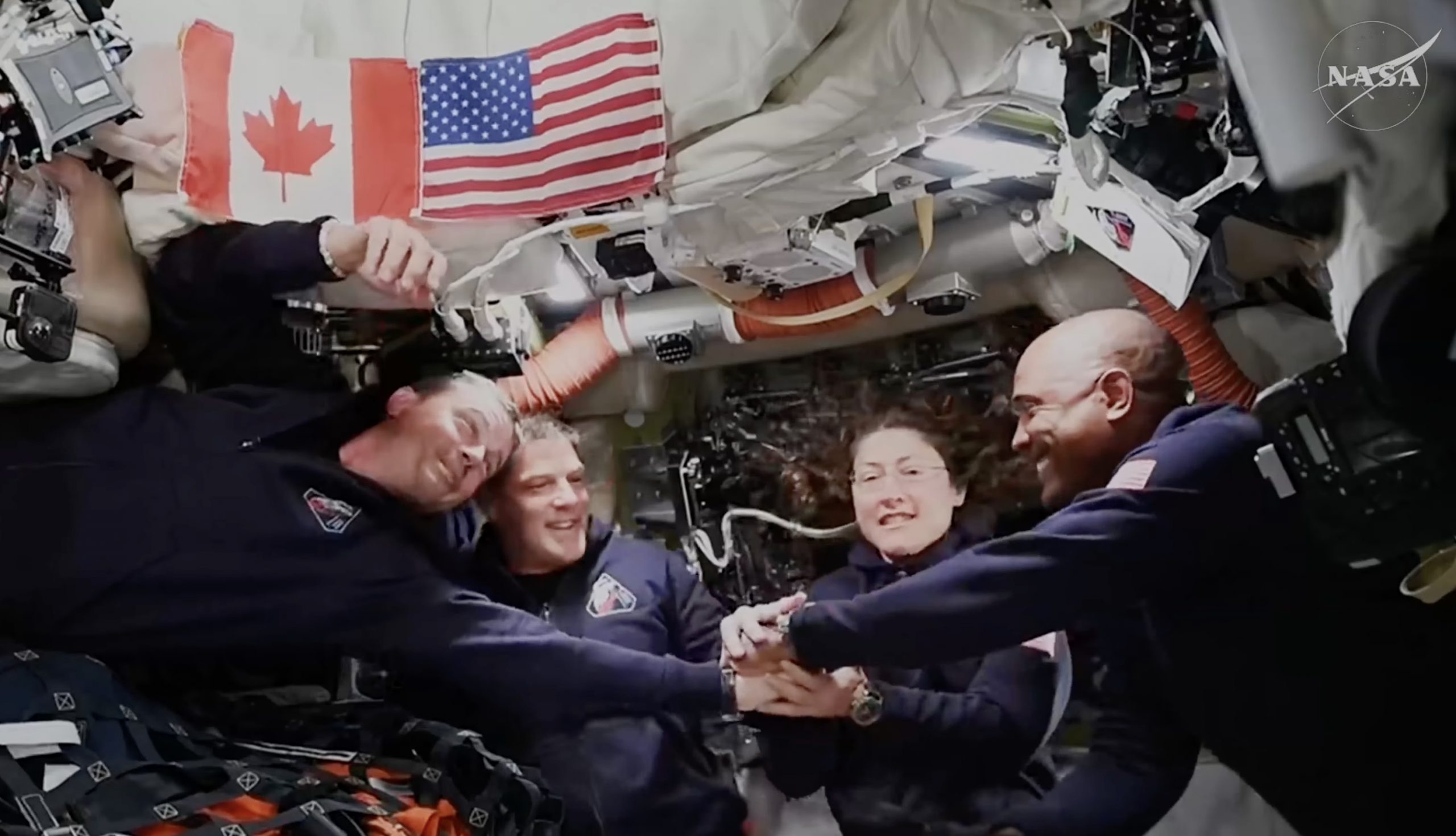
Carrying the torch from Apollo, through shuttle and station, to a hoped-for new era of space exploration, the Artemis 2lunar flyby exceeded expectations
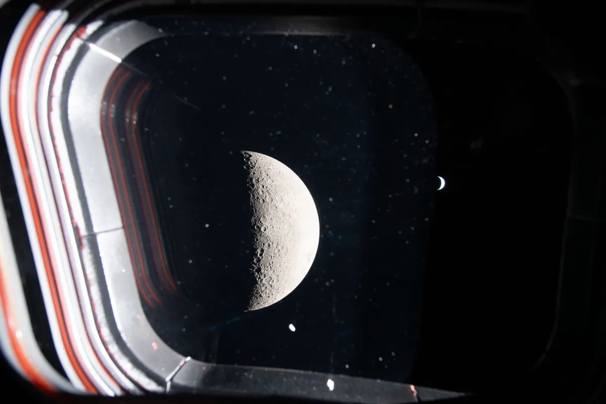
All last week I monitored the NASA mission coverage livestream. As the flyby approached, the Moon (Luna) waned from gibbous to half to crescent in just a few hours, while its apparent size grew to a basketball’s held at arm’s length. Earth appeared to set and rise. And then, partially lit by earthshine, haloed by the solar corona, floating in the void of space spangled with stars, amidst a parade of planets bathed in zodiacal light, the Moon eclipsed the Sun (Sol) and commander Reid Weisman declared, “We have not evolved to see such a sight.” Up until then, the crew photographs had done justice to their experiences, but no longer.
Responding to the astronauts waxing poetic and ecstatic, one capsule communicator, channelling Project Hail Mary‘s fictional Rocky, replied, “Amaze, amaze, amaze,” while another cap com replied, “Copy, moon joy.”
The crew travelled farther from Earth than any other humans, over a quarter million miles, about 1.3 light-seconds, when pilot Victor Glover advised, “Let’s actually savor the com delay we have.”
NASA Associate Administrator Amit Kshatriya remarked, “The [crew’s] expressions of love and devotion to family … is a great example of why we go and do these missions. If you can’t take love to the stars, then what are we doing? … why do we even go? That’s why we send humans instead of robots, [for] that firsthand witness. They’ll go through a whole range of emotions, like we who are watching them, and that’s the whole point: that we can share that experience.”
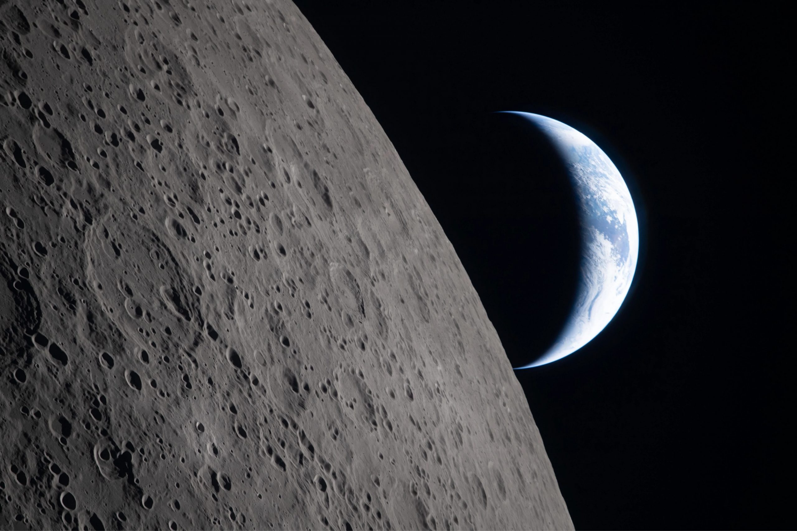
Half Moon and crescent Earth outside the window of the Artemis 2 Orion crew capsule “Integrity”.
Earth appears to set as the Artemis 2 crew moves behind the Moon. The lunar surface is comparatively dark and Earth is so bright it was difficult to look at.
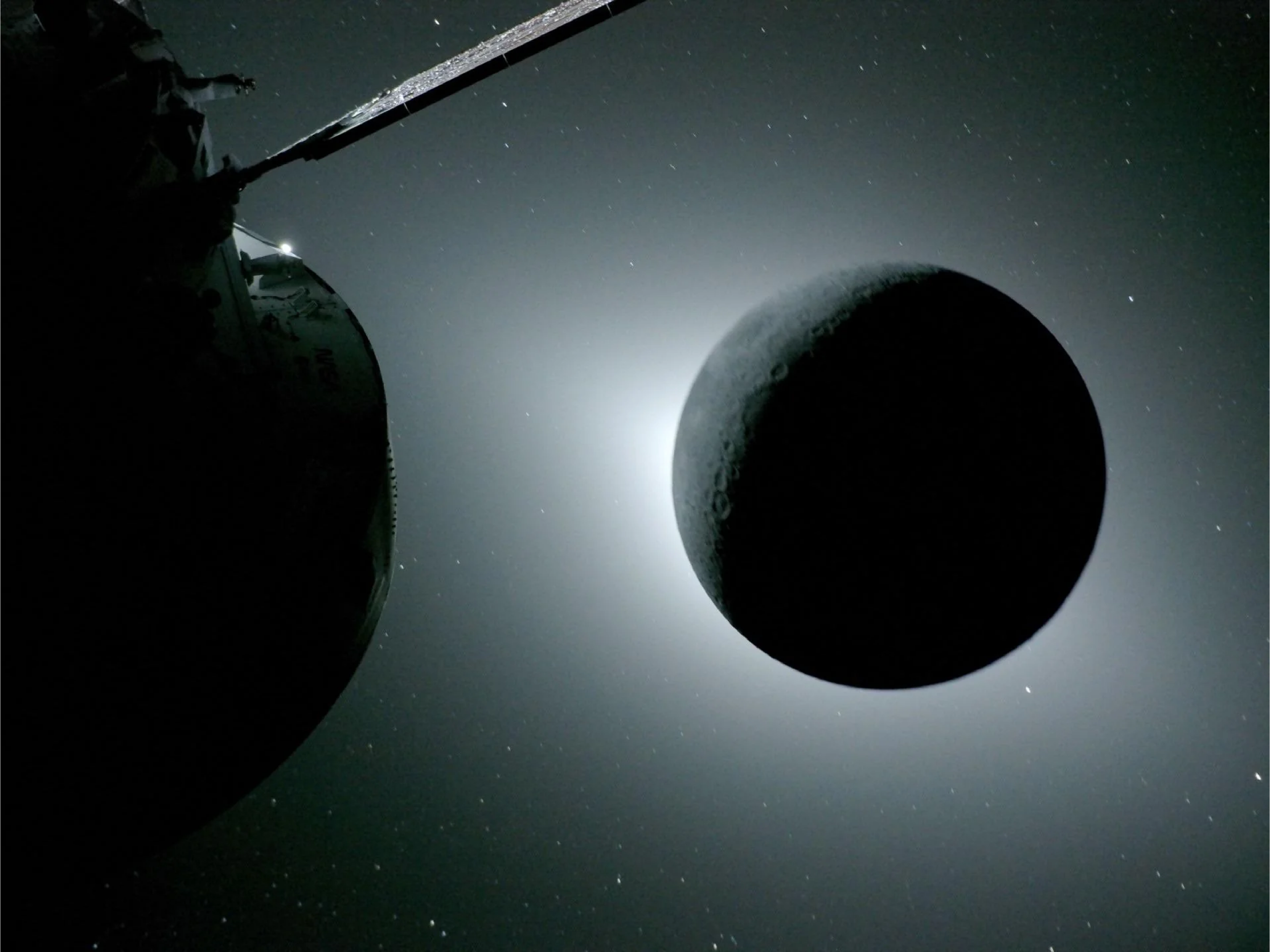
The Sun eclipsed by the Moon (right) as seen by Artemis 2 (left) from a camera at the end of one of its solar arrays. The Moon is partially lit by Earthshine (upper left, out of frame) with Venus (upper left, nearly eclipsed by the spacecraft) and Saturn and Mars (lower right) amidst stars of the constellation Pisces.
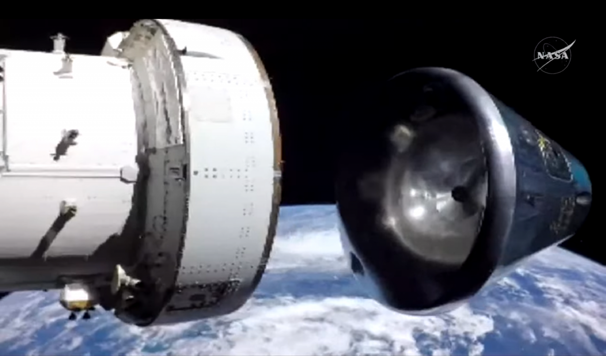
Broadcast live, ESA’s service module (left) separates from NASA’s command module (right) with the crew shortly before Artemis 2’s atmospheric reentry, again recorded from a solar array end.
As a child of the Apollo program and a lifelong dreamer of spaceflight, I am thrilled to follow the Artemis 2 mission, carrying the first humans around the Moon (Luna) in over half a century, with the intent to pick up where we left off, establish a permanent lunar presence, and proceed to Mars and beyond.
This evening, the Artemis 2 crew of ReidWiseman, VictorGlover, Kristina Koch, and JeremyHansen approaches the Moon’s gravitational sphere of influence, where lunar gravity exceeds terrestrial gravity. Kristina recently remarked, “Our strong hope is that this mission is the start of an era where everyone — every person on Earth — can look at the Moon and think of it as … a destination.” The dream is alive.
In Greek mythology, Artemis is the sister of Apollo; in reality, Artemis is safer (better computers), cheaper (as a fraction of US budget), and bigger (crew of 4 rather than 3) than Apollo. More importantly, with international and commercial help, I am hopeful that Artemis will evolve to a sustainable program so the Moon really does enter the human sphere as a destination, dramatically and irreversibly expanding the range of human experience.
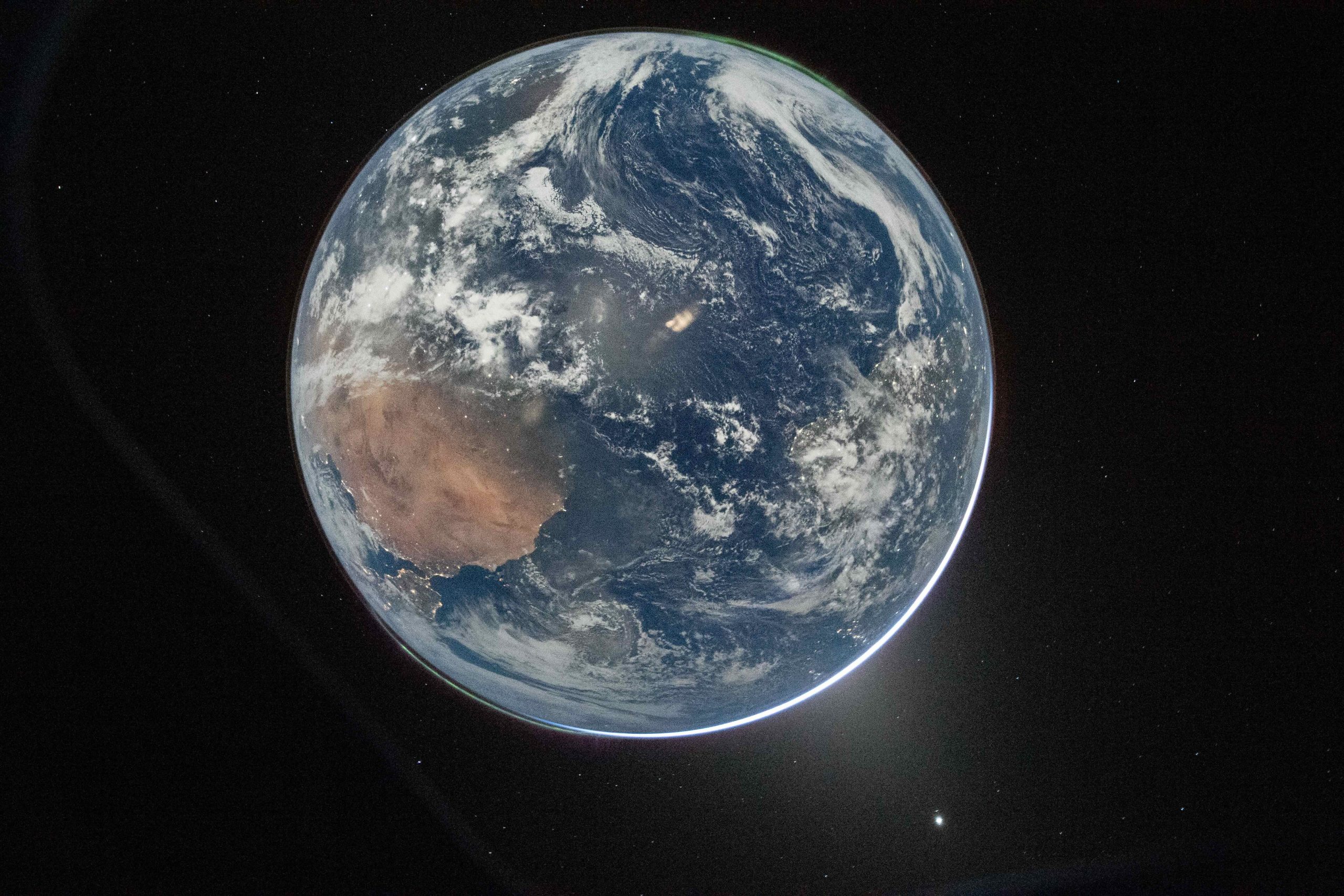
This Reid Wiseman Artemis 2 photo shows Earth illuminated by moonlight, except for a thin crescent illuminated by sunlight, with Venus in zodiacal light at 4 o’clock joined by aurora at 1 o’clock and 7 o’clock, shortly after translunar injection (TLI), 2026 April 2.
Artemis 2 crew — Reid, Jeremy, Kristina, Victor — in their Orion spacecraft “Integrity” en route to the Moon, 2026 April 4.
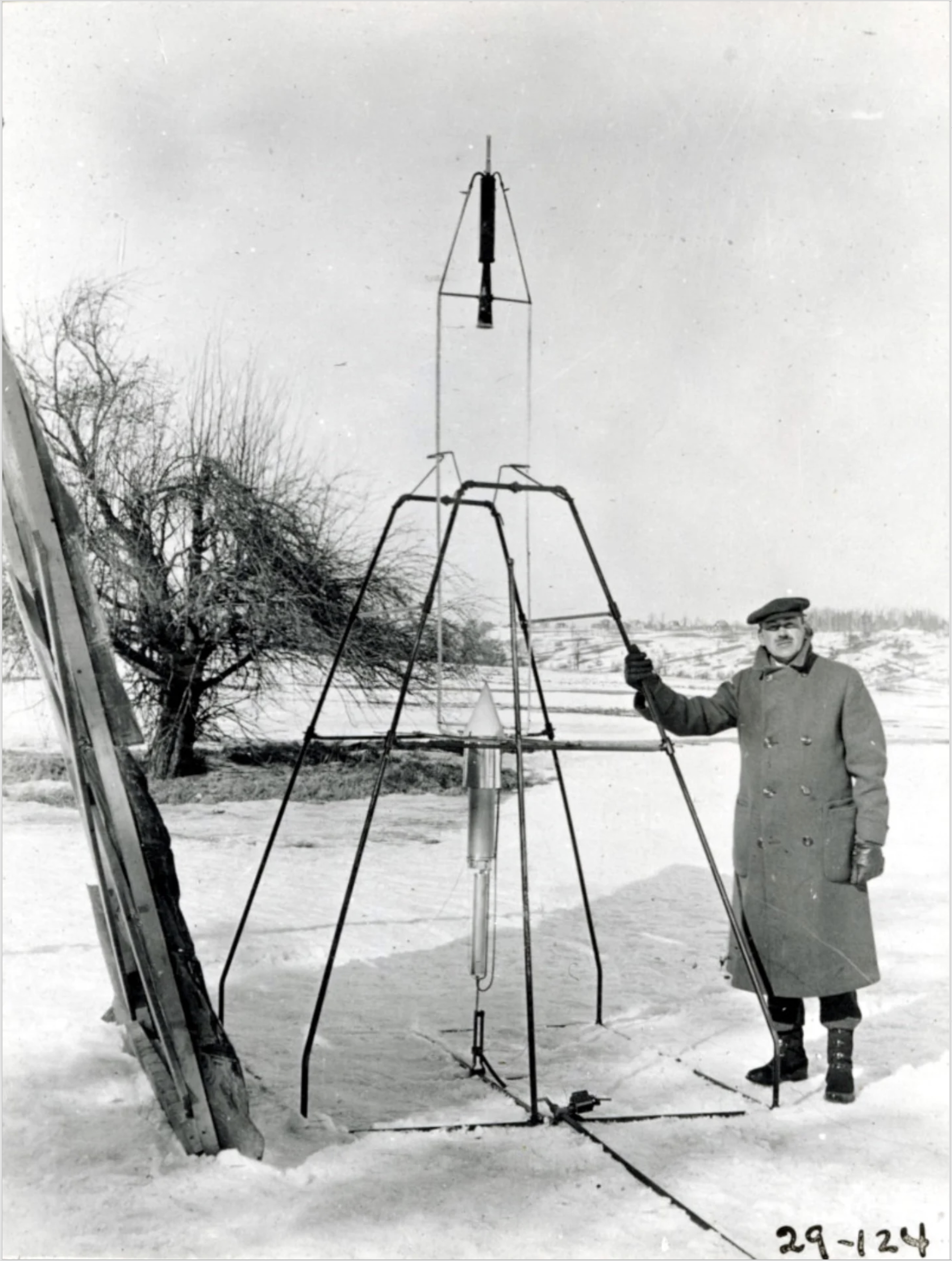
100 years ago, physicist Robert Goddard designed and built the first liquid-fueled rocket. Powered by gasoline and liquid oxygen and launched from his Aunt Effie’s farm in Auburn, Massachusetts on 1926 March 16, the first flight lasted 2.5 seconds and reached an altitude of 12.5 meters.
7 years earlier, in 1919, Goddard published the seminal treatise A Method of Reaching Extreme Altitudes, whose final section is “Calculation of minimum mass required to raise one pound to an ‘infinite’ altitude”, including to the Moon. Goddard eschewed publicity, but his ideas were nonetheless widely ridiculed.
In 1920, an unsigned New York Times editorial denied that a rocket could work in a vacuum and suggested that Goddard “seems to lack the knowledge ladled out daily in high schools.” In 1929, a local newspaper mocked one of Goddard’s experiments with the headline “Moon rocket misses target by 298,799 ½ miles”.
Goddard remarked, “It is difficult to say what is impossible, for the dream of yesterday is the hope of today and the reality of tomorrow.”
Robert Goddard did not live to see the Space Age he helped create, but his wife Esther Goddard, who championed his work after his death, did live to see the 1969 July 16 launch of Apollo 11, which used a liquid-fueled rocket based on principles pioneered by him to reach the Moon. The crew included Buzz Aldrin, the son of one of his students.
The day after Apollo 11 launched, the New York Times corrected its 1920 error and acknowledged that rockets can fly in a vacuum (by expelling mass in one direction and recoiling in the opposite direction).
Robert Goddard and the first liquid-fueled rocket on 1926 March 8. (The combustion chamber is above the propellant tanks, but he reversed the order in later versions.) Photo by Esther Goddard.
Yuhe Ren, Niklas Manz, and I recently published an article Guided flame: reaction-diffusion of fire pulses in narrow channels in the journal Open Transport. Tim Siegenthaler helped machine the channels. This work had been gestating for a long time but has recently became a hot topic. Fortunately, Yuhe was able to acquire all our data in the last year, spanning his Junior I.S., Wooster summer REU (thanks to the KoontzEndowed Fund), and Senior I.S.
We studied fire propagation in annular channels whose rectangular cross-sections are a few millimeters wide and high and whose circumferences are hundreds of millimeters long. If a channel is partially filled with a volatile flammable hydrocarbon fluid, locally igniting the vapor above the fluid can start a fire pulse that rapidly propagates around the annulus at hundreds of millimeters per second leaving behind an unexcitable region of depleted vapor, a refractory tail. Further evaporation of the volatile fluid restores the vapor and the corresponding excitable condition, allowing the returning pulse to propagate, provided the channel’s circumference is sufficiently long.
Experimentally, we explored this quasi-one-dimensional reaction-diffusion system, discovering simple trends connecting refractory tail length and pulse propagation speed to channel length, height, and width. Computationally, we introduced phenomenological computer simulations that simply reproduce the guided flame and elucidate the underlying physics.
Yuhe’s overhead video of a blue hydrocarbon flame propagating at almost one meter per second counterclockwise in a narrow channel in a fume hood. (You may need to click or tap to see the motion.)
As command module pilot for the 1971 Apollo 14 mission, Stuart Roosa was one of 24 people to travel around the Moon* in the heroic first age of lunar exploration. He was also a former U.S. Forest Service smokejumper, and he carried into lunar orbit about 500 seeds to test the effects of spaceflight on the resulting trees. Upon returning to Earth, almost all the seeds germinated successfully, and many of the seedlings were distributed widely for the 1976 U.S. Bicentennial. After 50 years, no differences have been noted between Moon trees and Earth trees.
NASA repeated this experiment for the 2022 Artemis I test flight. While we await the next 4 people to travel around the Moon, during Artemis II later this year, I recently visited Asheville Botanical Garden to see its Apollo Moon Tree. It was a clear and unseasonably warm February day, and I found the sycamore barren of leaves but apparently healthy, only distinguishable by the plaque at its base.
*Luna is arguably a better name for Earth’s natural satellite.
At the Asheville Botanical Garden with a sycamore tree planted from a seed that travelled around the moon with astronaut Stuart Roosa during Apollo 14 in 1971.
Recent Comments
Thanks, Mark! I enjoy reading your posts as well.
Nice post, John! Thanks for writing these. I always enjoy them.


Thanks, Mark! I enjoy reading your posts as well.