Not only can suns stand still in the sky, from some exoplanets their motion can apparently reverse! Wooster physics-math double majors Xinchen (Ariel) Xie ’21 and Hwan (Michelle) Bae ’19 and I just published an article elucidating these apparent solar reversals.
Michelle and I began studying the architecture of daylighting terrestrial buildings for energy efficiency as part of her senior thesis, but due to our mutual interests, we gravitated to extraterrestrial possibilities. After my return from a yearlong sabbatical, Ariel eagerly continued the work for her senior thesis. Despite a pandemic keeping us a planet apart and meeting via video conference at simultaneously very early and very late hours, we completed the project, one of the most beautiful in my 33 years at Wooster. During one of our early morning, late evening sessions, we mathematically derived the solar reversals condition for the important special case of zero obliquity or tilt.
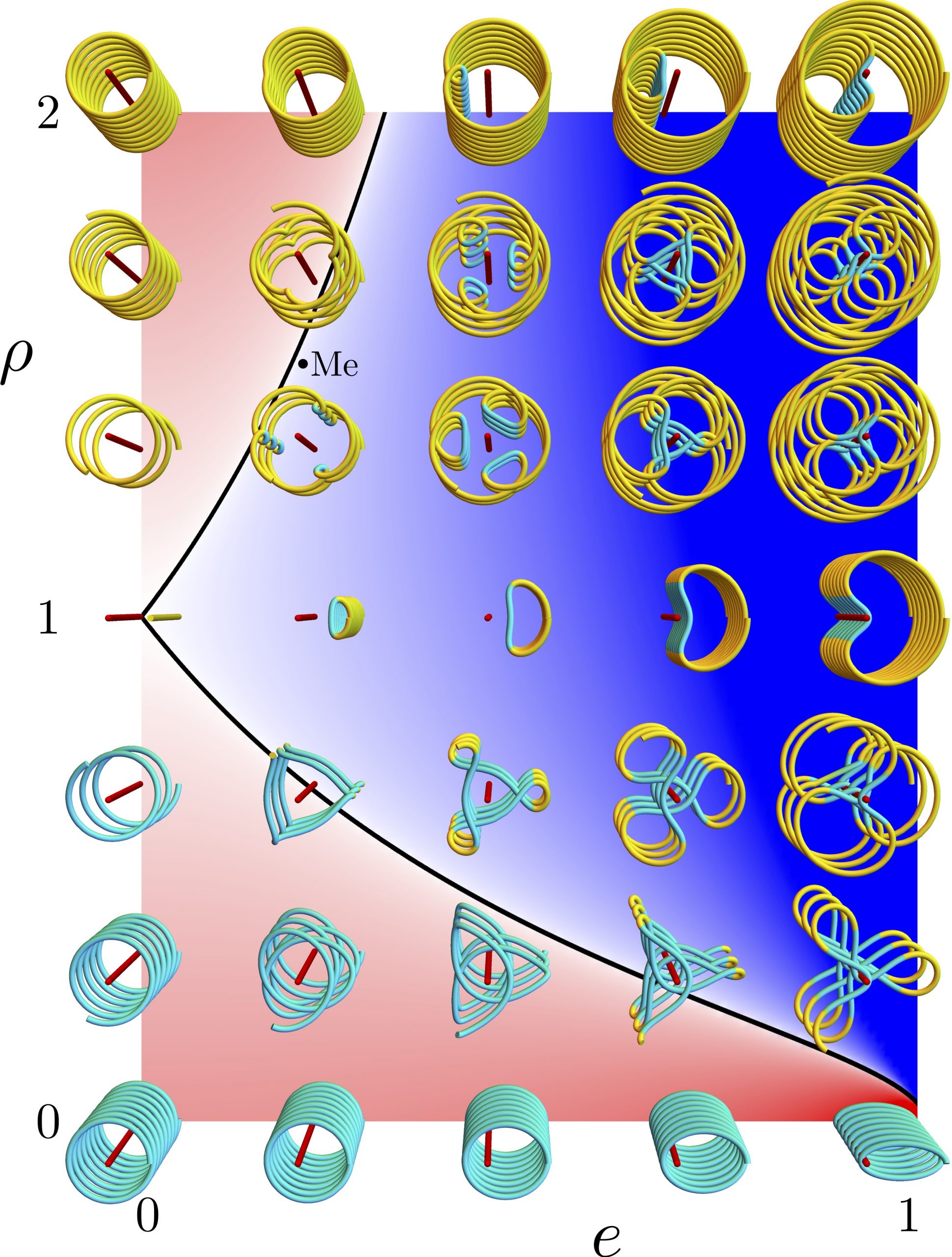
In the first figure below, exoplanet spin-orbit ratio \rho increases rightward, orbital eccentricity e increases upward, and time t increases outward. Red rods represent planetary observers, and coils represent apparent position and angle of their suns for 8 orbits. Yellow and cyan indicate apparent clockwise and counterclockwise motion, which signify reversals in coils with both colors. Our own solar system’s Mercury (Me) is just inside the reversal region. Red-white-blue background colors represent the product of the differences of the planet’s spin angular speed and its extreme orbital angular speeds at apoapsis and periapsis; red means no apparent solar reversals, blue means reversals, and the saturation indicates the reversal magnitude.
On Mercury, one (solar) day lasts two years, and once a year an equatorial observer witnesses a brief solar reversal, as in the second figure below, surely a special day for any future inhabitants. For a civilization inhabiting such a planet, we expect “reversal day” to be culturally significant.
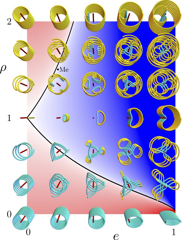
Apparent solar motion for different spin-orbit ratios and orbital eccentricities; red background means no apparent solar reversals, blue means reversals, and saturation indicates the reversal magnitude.
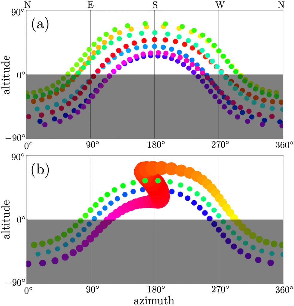
Solar strobe plots. (a) Earth-like planet whose sun appears to rise in the east and set in the west every day; rainbow hues code time. (b) Mercury-like exoplanet whose sun appears to reverse its motion once a year near periapsis where it appears largest.


![Star (red) and planet (cyan) gravitationally pull a mass (orange) into a halo orbit (yellow).[You may need to click to see the animation.]](http://woosterphysicists.scotblogs.wooster.edu/files/2022/08/halo9.gif)